Machine Learning is the crucial part of Data Scientist’s interview, because this skill is like the Force for a Jedi master. -Bruce Yang
In the first few rounds of Data Scientist interview, most companies will heavily focus on your machine learning knowledge (the breadth of machine learning), to test how many algorithms you are familiar with and used in real life projects. I summarize the top 15 algorithms and the 5 most commonly asked questions (The Big Five).
The Big Five
- What are the basic concepts? What problem does it solve?
- What are the assumptions?
- What are the steps of the algorithm?
- What is the cost function?
- What are the advantages/disadvantages?
Practical Machine Learning Questions and Top 15 Machine Learning Algorithms Summary
Contents
- 1 Practical Machine Learning Questions
- 2 Linear Regression
- 3 Regression with Lasso
- 4 Regression with Ridge
- 5 Logistic Regression
- 6 Naïve Bayes
- 7 K-Nearest Neighbors
- 8 K-means Clustering
- 9 Decision Tree
- 10 Random Forest
- 11 Ada-Boost
- 12 Gradient Boosting
- 13 SVM (Support Vector Machine)
- 14 PCA (Principal Component Analysis)
- 15 Neural Networks
Topics
- 1.1 What is Bias-Variance Tradeoff?
- 1.2 What is the curse of dimensionality?
- 1.3 What is Multi-Collinearity? Why is it an issue?
- 1.4 How do you detect multicollinearity in Model Data?
- 1.5 What are the remedies of problem of Multi-collinearity?
- 1.6 What are Outliers? Leverage & Influential points?
- 1.7 How can we deal with Outliers?
- 1.8 Why do you need Cross-Validation?
- 1.9 How to detect overfitting?
- 1.10 How do you handle overfitting problem?
- 1.11 How to handle missing data?
- 1.12 You have a train-set, a dev-set and a test-set, how did you manage the distribution of those sets?
- 1.13 How to handle imbalanced data?
- 1.14 What are the methods for over-sampling?
- 1.15 What is Confusion Matrix? What’s TP, TN, FP, FN, Precision and Recall?
- 1.16 What is ROC and AUC?
- 1.17 What are the different types of variables? How to handle categorical variables? Are rare labels in a categorical variable a problem?
- 1.18 Are rare labels in a categorical variable a problem?
- 1.19 Why cardinality can cause overfitting?
- 1.20 What is the difference between Generative models and Discriminative models?
Section 1. Pratical Machine Learning Questions
1.1 What is Bias-Variance Tradeoff?
Bias:
- The difference between the predicted values and the true values. Bias is the difference between the average prediction of our model and the correct value which we are trying to predict.
- High bias can cause an algorithm to miss the relevant relations between features and target outputs.
- Model with high variance pays a lot of attention to training data and does not generalize on the data which it hasn’t seen before. As a result, such models perform very well on training data but has high error rates on test data.
- For example, if you want to predict the entire country’s house price, but you are only use New York’s data to build the model, that means your model is biased.
Variance:
- The difference between the predicted values. Variance is the variability of model prediction for a given data point.
- Variance is a type of error that occurs due to a model’s sensitivity to small fluctuations in the training set.
- High variance can cause an algorithm to model the random noise in the training data, rather than the intended outputs.
- You trained a good complex model on your training data, but when you do the prediction on the testing data, the accuracy becomes very low.
Error \( e \):
Let's assume that we are modeling the relationship between Y and X
\[ Y = f(X) + e \]
Where \( e \) is the error term and it's normally distributed with a mean of 0.
So the expected squared error at a point x is:
\[ Err(x) = E[(Y-\hat{f}(x))^2] \]
\[ Err(x) = (E[\hat{f}(x)]-f(x)])^2 + E[(\hat{f}(x)-E[\hat{f}(x)])^2] + \sigma^2 \]
\[ Err(x) = Bias^2 + Variance + Irreducible Error \]
Irreducible error is the error that can’t be reduced by creating good models. It is a measure of the amount of noise in our data.
Under-fitting: happens when a model is unable to capture the underlying pattern of the data. These models have high bias and low variance. For example, when we try to build a linear model with a nonlinear data.
Over-fitting: happens when our model captures the noise along with the underlying pattern in the data. These models have low bias and high variance.
Trade-off: basically we need to find the right balance without overfitting and underfitting. If our model is too simple and has very few parameters then it may have high bias and low variance. On the other hand, if our model has a large number of parameters then it will have a high vairance and low bias.
To build a good model, we need to find a good balance between bias and variance such that it minimizes the total error.
1.2 What is the curse of dimensionality?
If we have more features than observations then we run the risk of massively overfitting our model — this would generally result in terrible out of sample performance.
High-Dimensionality = Sparsity, Sparsity = Error. For example, the K observations that are nearest to a given test observation \(x_{0}\), it may be very far away from \(x_{0}\) in p-dimensional space when p is large, leading to a very poor prediction of f. Machine learning’s basic strategy is to make inferences by looking at similar data.
If the distances are all approximately equal, then all the observations appear equally alike (as well as equally different), and no meaningful information can be formed.
1.3 What is Multi-Collinearity? Why is it an issue?
- When independent variables in a multiple regression model are highly correlated. For example, if we are trying to use earnings report to predict stock returns, we put Assets, Liabilities, Owner’s (or Stockholders’) Equity together into the model, the multi-collinearity will happen.
- One variable is a linear combination of two or more variables.
- It increases the variance of the regression coefficients, making them unstable.
- One definition of Collinearity is that it is the extent to which a small change in the input creates a large change in the model
- It can be difficult to separate out the individual effects of collinear variables on the response, it’s hard to determine how each one separately is associated with the response
- Fail to reject H_{0}
1.4 How do you detect multicollinearity in Model Data?
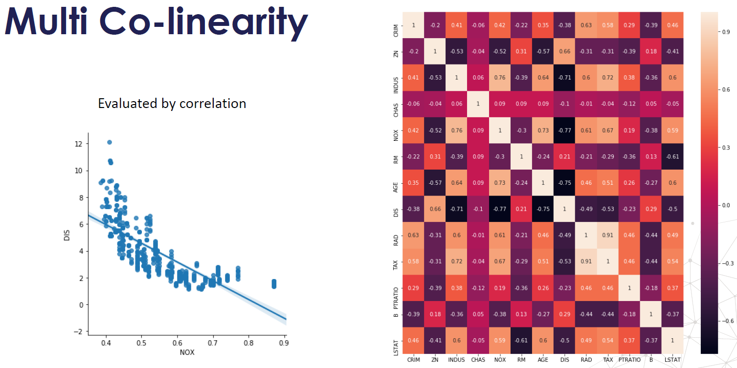
- Check Correlation Matrix
- Find out Variance Inflation Factor (VIF)-how much variance of the estimates gets inflated because of high collinearity.
- VIF is the ratio of the variance of beta when fitting the full model divided by the variance of beta if fit on its own the smallest possible value for VIF is 1, which indicates the complete absence of collinearity.
- VIF = 1 (OK); VIF < 5 (small warning); VIF >=5 & <= 10 (Strong Warning); VIF > 10 (Unacceptable)
- Partial Dependence Plots
1.5 What are the remedies of problem of Multi-collinearity?
- Drop one of the correlated variable — which one to drop? To see which one has more significance, drop less importance variable (to business team)
- Use PCA
- Use Partial Least Square
- Transform: add together
- If multicollinearity is found in the data, centering the data (that is deducting the mean of the variable from each score) might help to solve the problem. However, the simplest way to address the problem is to remove independent variables with high VIF values.
1.6 What are Outliers? Leverage & Influential points?
Outliers:
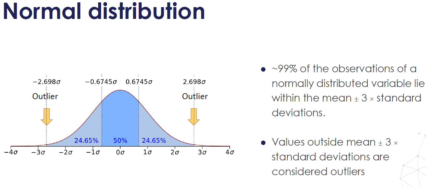
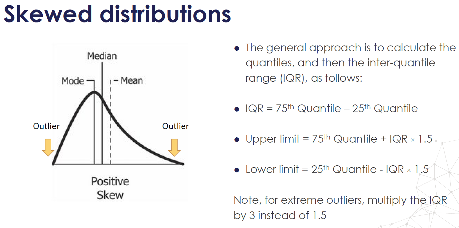
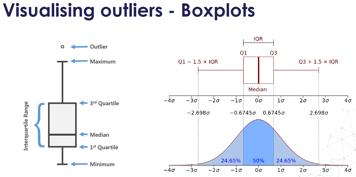
- Definition of Outliers (Benchmark): Outliers < Q1–1.5*IQR (Q3-Q1) or Outliers > Q3 + 1.5*IQR
- Wrong rule: 2 standard deviations rule, remove values 2 standard deviations away from the mean
Leverage:
- Definition of Leverage point: Points with extreme values of X are said to have high leverage.
- A data point that has an x-value far from the mean of the x-values is said to have high leverage. Deviate from the mean of X, 2 sd away.
- Slope and intercept may be largely unaffected, a person who is really tall and weights a lot may fit the overall pattern perfectly
Influence Point:
- Definition of Influence point: changed the slope a lot
- If the parameter estimates change a great deal when a point is removed from the calculations, the point is said to be influential.
Cook's Distance: how much the parameter estimates change when a point is removed from the calculations
\[ \frac{1}{n} + \frac{(X_{i}-\bar{X})^2}{SS_{XX}} \]
1.7 How can we deal with Outliers?
- Trimming: delete data when it is typographical errors or measurement error or contaminated distribution (want mid-level salary got some senior-level salary)
- Winsorizing: assigning outlier the next highest or lowest value found in the sample that is not an outlier; done when small amounts of scores are legitimate outliers; when you believe you are dealing with a valid data point derived from a heavy-tailed distribution.
- Trimming or Winsorizing greater than 5% may affect the outcome results: reduce power of analysis; makes ample normalcy of data; consider transforming data, choosing an alternate outcome variable or data analysis techinique
1.8 Why do you need Cross-Validation?
- CV can reduce model performance variance
- Cross Validation is used to assess the predictive performance of the models and and to judge how they perform outside the sample to a new data set also known as test data.
- Parameters Fine-Tuning
1.9 How to detect overfitting?
- Performs great on training data, but acts bad on testing data.
- The plot of training loss continues to decrease with experience.
- The plot of validation loss decreases to a point and begins increasing again.
1.10 How do you handle overfitting problem?
- Get more training data: so the model will become more generalized.
- Remove irrelevant features: do more feature selection
- Early Stopping: is a form of regularization used to avoid overfitting when training a learner with an iterative method, such as gradient descent. Such methods update the learner so as to make it better fit the training data with each iteration.
- Regularization: for example, you could prune a decision tree, use dropout on a neural network, or add a penalty parameter to the cost function in regression.
1.11 What are the types of missing data? How to handle missing data?
Types of missing data:
Missing data Completely at Random (MCAR):
- The probability of being missing is the same for all the observations.
- When data is MCAR, there is absolutely no relationship between the data missing and any other values, observed or missing, within the dataset. In other words, those missing data points are a random subset of the data. There is nothing systematic going on that makes some data more likely to be missing than other.
- If values for observations are missing completely at random, then disregarding those cases would not bias the inferences made.
Missing data at Random (MAR):
- The probability of an observation being missing depends on available information. It depends on other variables in the dataset
- For example, if men are more likely to disclose their weight than women, then weight is missing at random. More missing values for women than for men.
Missing data not at Random (MNAR):
- There is a mechanism or a reason why missing values are introduced in the dataset.
- For example, MNAR would occur if people failed to fill in a depression survey because of their level of depression. Here, the missing of data is related to the outcome, depression. We need to flag those missing values, good at prediction.
- Similarly, when a financial company asks for bank and identity documents from customers in order to prevent identity fraud, typically, fraudsters impersonating someone else will not upload documents, because they don't have them, because they are fraudsters. Therefore, there is a systematic relationship between the missing documents and the target we want to predict: fraud.
Handle missing data:
Delete: you can drop variables if the data is missing like for more than 60% observations.
Impute: mean, median or mode is a very basic imputation method (rolling window or overall); predict the missing values with other independent variables using random forest. For categorical data, we can treat the missing values as a separate category by itself.
Mean or Medium imputation:
- When to use: when data is missing completely at random, no more than 5% of the variable contains missing data
- If the variable is normally distributed the mean and median are approximately the same
- If the variable is skewed, the median is a better representation.
Mode imputation:
- When to use: when data is missing completely at random, no more than 5% of the variable contains missing data
Missing category imputation:
- Easy to implement
- Fast way of obtaining complete datasets
- Can be integrated in production during model deployment
- Captures the importance of missingness if there is one
- No assumption made on the data
Missing indicator:
- Data is not missing at random.
- Missing data are predictive
- Many missing indicators may end up being identical or very highly correlated
1.12 You have a train-set, a dev-set and a test-set, how did you manage the distribution of those sets?
- Training set: Which you run your learning algorithm on.
- Dev (development) set: Which you use to tune parameters, select features, and make other decisions regarding the learning algorithm. Sometimes also called the hold-out cross validation set.
- Test set: which you use to evaluate the performance of the algorithm, but not to make any decisions regarding what learning algorithm or parameters to use.
- The purpose of the dev and test sets are to direct your team toward the most important changes to make to the machine learning system.
- Dev and Test sets should come from the same distribution, and it must be taken randomly from all the data.
- Choose dev and test sets to reflect data you expect to get in the future and want to do well on. The problem with having different dev and test set distributions: There is a chance that your team will build something that works well on the dev set, only to find that it does poorly on the test set. For example, ask your friends to take mobile phone pictures of cats and send them to you. Once your app is launched, you can update your dev/test sets using actual user data.
- Having mismatched dev and test sets makes it harder to figure out what is and isn’t working, and thus makes it harder to prioritize what to work on.
- As for the training data, you can generalize it as much as you can, under-sample or over-sample, but the dev/test set should reflect the real population (reflect what you ultimately want to perform well on, rather than whatever data you happen to have for training)
1.13 How to handle imbalanced data?
- Under-sampling: randomly sample the majority class down to match the minority class.
- Over-sampling: sample the minority class up to match the majority class.
1.14 What are the methods for over-sampling?
1.15 What is Confusion Matrix? What’s TP, TN, FP, FN, Precision and Recall?
- Confusion Matrix: to describe the performance of a classification Model
- TP: True Positive, predict class 1 and actual class 1.
- TN: True Negative, predict class 0 and actual class 0.
- FP: False Positive, predict class 1 but actual class 0 (False Alarm).
- FN: False Negative, predict class 0 but actual class 1.
- Precision: TP/(TP+FP).
- Recall: TP/(TP+FN).
1.16 What is ROC and AUC?
- ROC curve: it is a plot of the True Positive Rate v.s. the False Positive Rate for every possible classification threshold.
- True Positive Rate (Sensitivity): TP/(TP+FN)
- False Positive Rate: FP/(TN+FP)
- True Negative rate (specificity): TN/(TN+FP)
- AUC: is the area under the ROC curve, the larger the better. when AUC is 0.5, it means model has no class separation capacity whatsoever, equals randomly guessing.
Advantages of using ROC and AUC:
- There is a huge benefit of using an ROC curve to evaluate a classifier instead of a simpler metric such as misclassification rate.
- ROC curve visualizes all possible thresholds
- Misclassification rate is error rate for a single threshold
- AUC is a useful metric even when your classes are highly unbalanced.
1.17 What are the different types of variables? How to handle categorical variables?
Types of Variables:
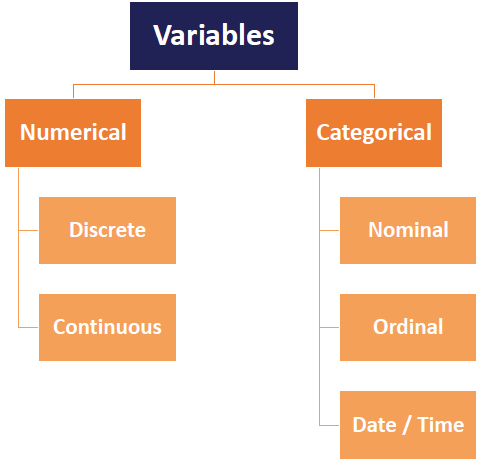
- Nominal data: use one hot encoding
- One-Hot-Encoding has the advantage that the result is binary rather than ordinal and that everything sits in an orthogonal vector space. The disadvantage is that for high cardinality, the feature space can really blow up quickly and you start fighting with the curse of dimensionality.
- Ordinal data: use label encoding
1.18 Are rare labels in a categorical variable a problem?
Rare values can add a lot of information or none at all. For example, consider a stockholder meeting where each person can vote in proportion to their number of shares. One of the shareholders owns 50% of the stock, and the other 999 shareholders own the remaining 50%. The outcome of the vote is largely influenced by the shareholder who holds the majority of the stock. The remaining shareholders may have an impact collectively, but they have almost no impact individually.
The same occurs in real life datasets. The label that is over-represented in the dataset tends to dominate the outcome, and those that are under-represented may have no impact individually, but could have an impact if considered collectively.
More specifically,
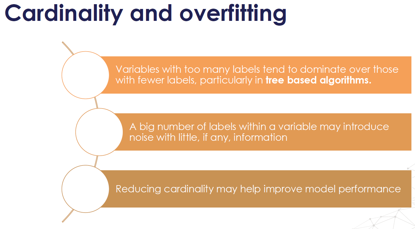
- Rare values in categorical variables tend to cause over-fitting, particularly in tree based methods.
- A big number of infrequent labels adds noise, with little information, therefore causing over-fitting.
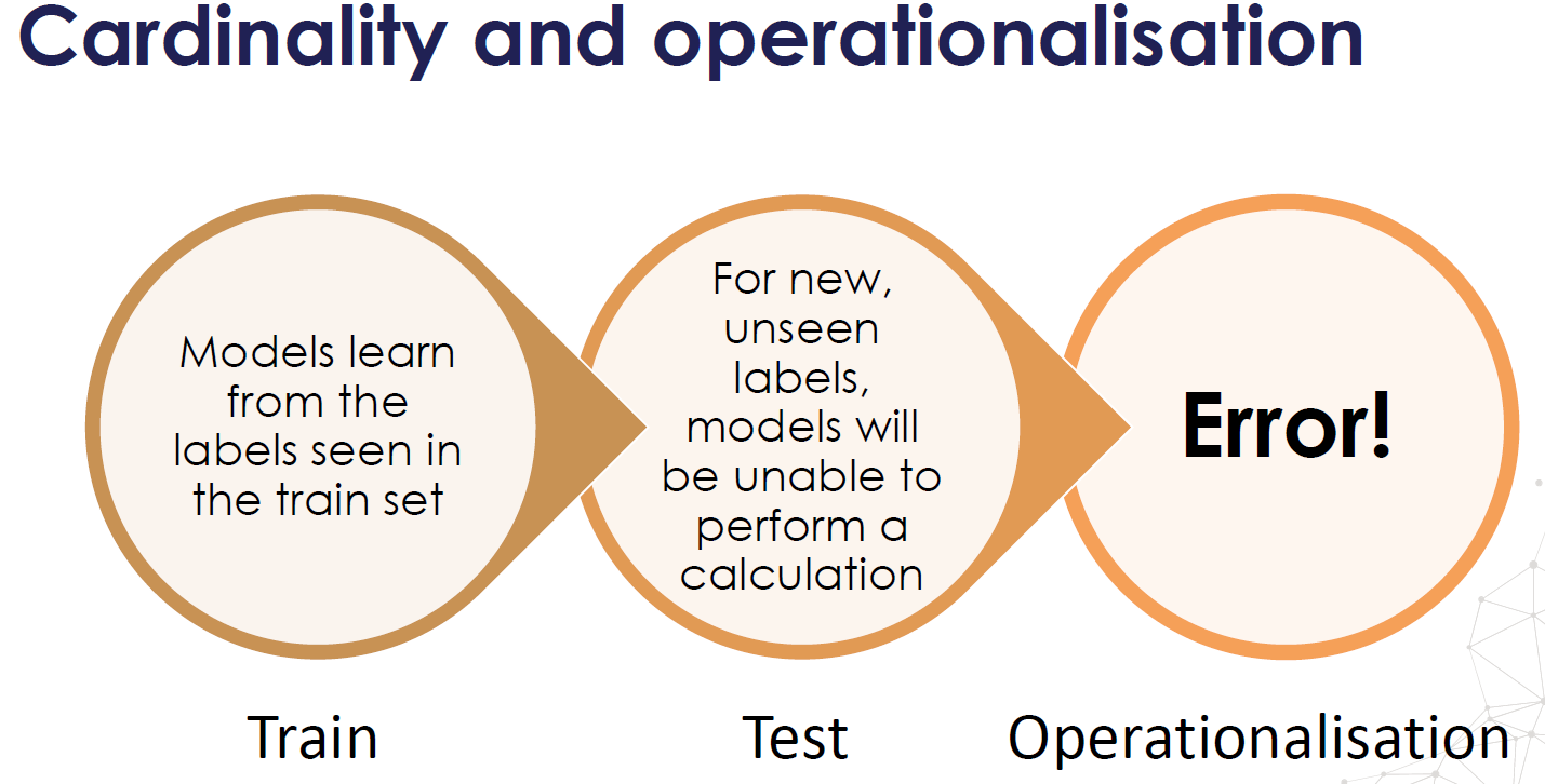
- Rare labels may be present in training set, but not in test set, therefore causing over-fitting to the train set.
- Rare labels may appear in the test set, and not in the train set. Thus, the machine learning model will not know how to evaluate it.
- One common way of working with rare or infrequent values, is to group them under an umbrella category called 'Rare' or 'Other'. In this way, we are able to understand the "collective" effect of the infrequent labels on the target.
**Note** Sometimes rare values, are indeed important. For example, if we are building a model to predict fraudulent loan applications, which are by nature rare, then a rare value in a certain variable, may be indeed very predictive. This rare value could be telling us that the observation is most likely a fraudulent application, and therefore we would choose not to ignore it.
1.19 Why cardinality can cause overfitting?
The number of different labels is known as cardinality
For highly cardinal variables, some labels may appear only in train set then over-fitting, some labels may appear only in test set, then model will not know how to interpret the values
1.20 What is the difference between Generative models and Discriminative models?
A Discriminative model models the decision boundary between the classes.
- Logistic Regression
- SVM
- Neural Networks
- Conditional Random Fields (CRF)
A Generative Model models the actual distribution of each class.
- Naïve Bayes
- Bayesian networks
- Markov random fields
- Hidden Markov Models (HMM)
Section 2. Linear Regression
2.1 What are the basic concepts? What problem does it solve?
Basic Concept: linear regression is used to model relationship between continuous variables. Xs are the predictor, explanatory, or independent variable. Y is the response, outcome, or dependent variable.
2.2 What are the assumptions?
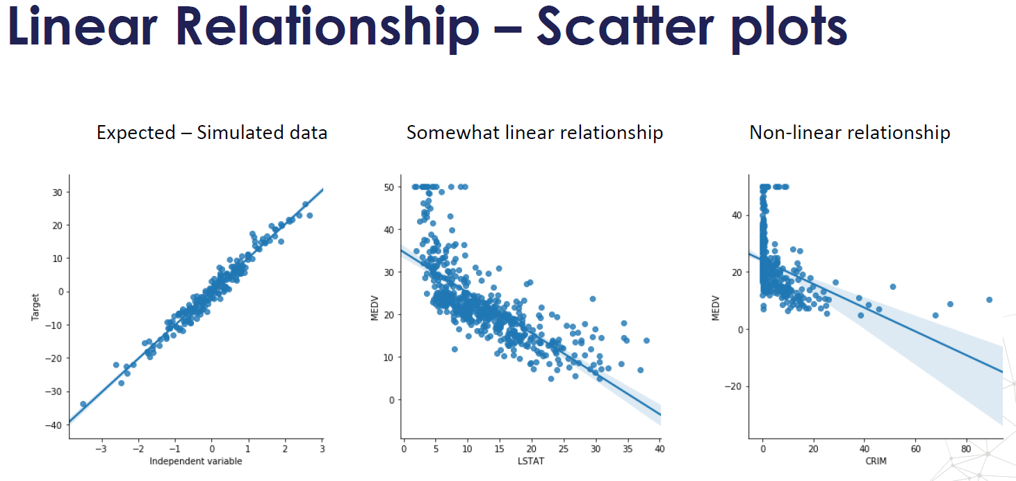
- Linearity: there is a linear relationship between the variables and the target. Linear relationship can be assessed with scatter plots.
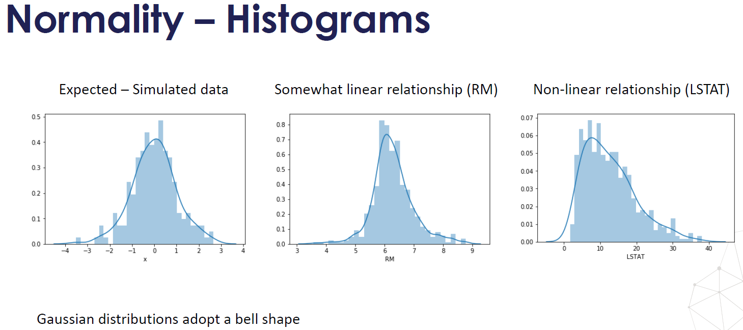
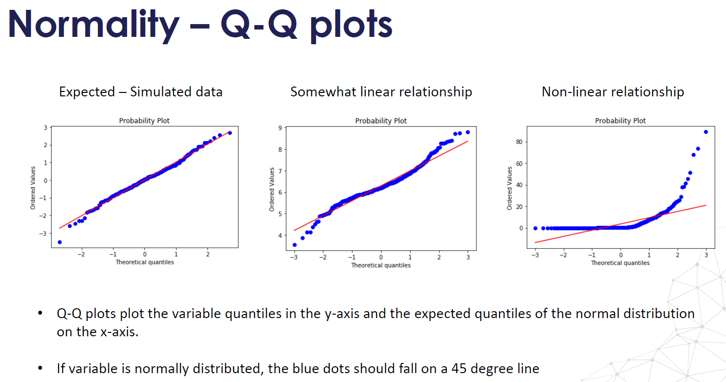
- Normality, variables follow a Gaussian Distribution, normality can be assessed with histograms and Q-Q plots. Normality can be statistically tested, for example with the Kolmogorov-Smirnov test. When the variable is not normally distributed a non-linear transformation like Log-transformation may fix this issue.
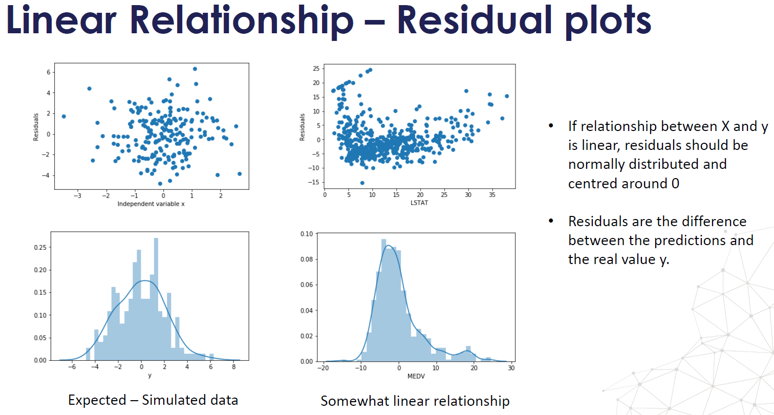
- Residuals are statistically independent, have uniform variance, are normally distributed
- The epsilon \(\epsilon\) term is assumed to be a random variable that has a mean of 0 and normally distributed
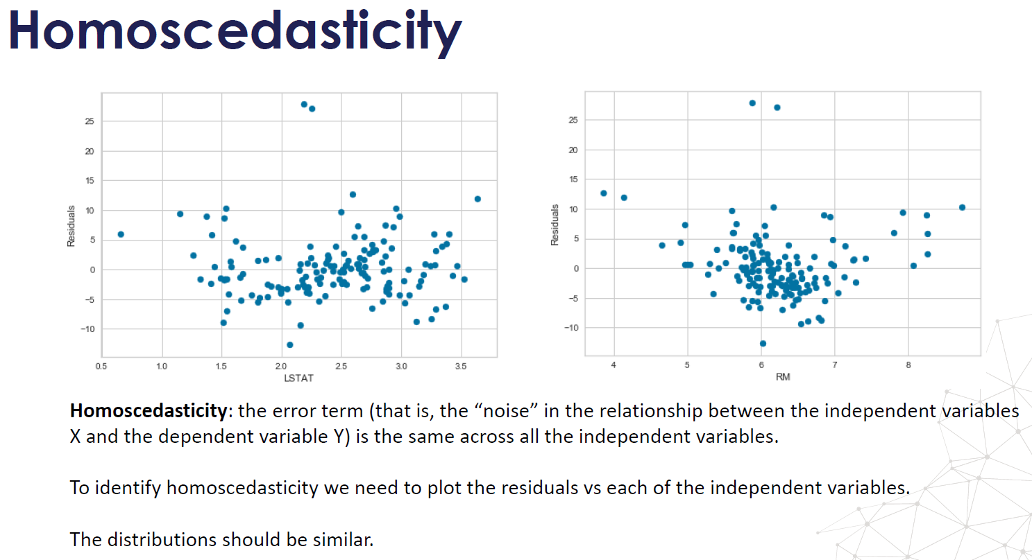
- Homoscedasticity: homegeneity of variance. The \(\epsilon\) term has constant variance \( \sigma^2 \) at every value of X (Homoscedastic). There are tests and plots to determine homescedasticity. Residual plots, Levene's test, Barlett's test, and Goldfeld-Quandt Test.
- The error terms are also assumed to be independent. \( \epsilon\) ~ \(N(0,\sigma^2) \)
- Non-collinearity: multicolinearity occurs when the independent variables are correlated with each other.
2.3 What if the errors are not normally distributed?
If the erros are not Gaussian distribution, we can still use linear regression, the only thing that is gonna be different is what you use for calculating coefficients, the calculating formula is biased if the errors are not normally distributed, because you are minimizing the MSE, if the errors are not Gaussian, then the maximum likelihood coefficients are not necessary the ones that come to minimize the MSE, you can still use linear regression.
2.4 What are the differences between erros and residuals?
- An error is the difference between the observed value and the true value (very often unobserved, generated by the DGP).
- A residual is the difference between the observed value and the predicted value (by the model).
- Error term is thus a theoretical concept that can never be observed, but the residual is a real-world value that is calculated for each observation every time a regression is run.
- Errors pertain to the true data generating process (DGP), whereas residuals are what is left over after having estimated your model. In truth, assumptions like normality, homoscedasticity, and independence apply to the errors of the DGP, not your model’s residuals. (For example, having fit 𝑝+1p+1 parameters in your model, only 𝑁−(𝑝+1)N−(p+1) residuals can be independent.) However, we only have access to the residuals, so that’s what we work with.
2.5 How to implement Linear Regression?
We want to find the best fit line: \[\hat{y_i} = b_0 + b_1 * x_i \]
We can achieve that by using least squares estimation, which minimizes the sum of the squared predicted errors.
We need to find the values of \( b_0\) and \( b_1\) that minimize:\[Q = \sum_{i=1}^{n} (y_i-\hat{y_i})^2 \] such that
\[b_1 = \frac{\sum_{i=1}^{n}(x_i-\bar{x})(y_i-\bar{y})}{\sum_{i=1}^{n}(x_i-\bar{x})^2} \] and \[ b_0 =\bar{y}- b_1\bar{x} \]
B1 = covariance(x, y) / variance(x)
B0 = mean(y) - B1 * mean(x)
2.6 What is the cost function of Linear regression?
\[ MSE = \frac{1}{n}\sum_{i=1}^{n} (y_i-\hat{y_i})^2 \]
2.7 If you have a set of data and do regression, what if you duplicate all the data and do regression on the new data set?
The mean and variance of the sample would not change therefore the beta estimation would be the same. The standard error will go down. However, since the sample size is doubled this will result in the lower p-value for the beta (from central limit theorem, the standard deviation of the sample mean = standard deviation of population / sqrt(n). This tells us that by simply doubling/duplicating the data, we could trick the regression model to have smaller confidence interval.
2.8 What is R^2?
- R² is called coefficient of determination.
- R² = variance explained by the model / total variance
- 0% represents a model that does not explain any of the variation in the response variable around it’s mean.
- 100% represents a model that explains all of the variation in the response variable around its mean.
- Usually, the larger the R², the better the regression model fits your observations.
2.9 What Is the Adjusted R-squared?
The adjusted R-squared compares the explanatory power of regression models that contain different numbers of predictors.
Suppose you compare a five-predictor model with a higher R-squared to a one-predictor model. Does the five predictor model have a higher R-squared because it’s better? Or is the R-squared higher because it has more predictors? Simply compare the adjusted R-squared values to find out! The adjusted R-squared is a modified version of R-squared that has been adjusted for the number of predictors in the model. The adjusted R-squared increases only if the new term improves the model more than would be expected by chance. It decreases when a predictor improves the model by less than expected by chance. The adjusted R-squared can be negative, but it’s usually not. It is always lower than the R-squared.
2.10 What’s Gradient Descent?
Gradient Descent is an optimization algorithm that helps machine learning models converge at a minimum value through repeated steps. Essentially, gradient descent is used to minimize a function by finding the value that gives the lowest output of that function. Often times, this function is usually a loss function.
2.11 How to implement Gradient Descent?
- Obtain a function to minimize F(x)
- Initialize a value x from which to start the descent or optimization from
- Specify a learning rate that will determine how much of a step to descend by or how quickly you converge to the minimum value
- Obtain the derivative of that value x (the descent)
- Proceed to descend by the derivative of that value multiplied by the learning rate
- Update the value of x with the new value descended to
- Check your stop condition to see whether to stop
- If condition satisfied, stop. If not, proceed to step 4 with the new x value and keep repeating algorithm
2.12 What’s the difference between confidence interval and predicted interval?
2.13 What are the Advantages/Disadvantages of Linear regression?
Pros:
- Simplicity and interpretability: linear regression is an extremely simple method. It is very easy to use, understand, and explain.
- The best fit line is the line with minimum error from all the points, it has high efficiency
- It needs little tuning
Cons:
- Linear regression only models relationships between dependent and independent variables that are linear. It assumes there is a straight-line relationship between them which is incorrect sometimes.
- Linear regression is very sensitive to the anomalies/outliers in the data
- Linear regression is very sensitive to missing data.
- Linear regression needs feature scaling.
- If the number of the parameters are greater than the samples, then the model starts to model noise rather than relationship
- Correlated features may affect performance.
- Extensive feature engineering required.
Section 3. Regression with Lasso
3.1 What are the basic concepts of Lasso? What problem does it solve?
Lasso is not a type of model, it is a regularization method for selecting variables and shrinking coefficients to adjust for complexity.
Lasso uses an L1 penalty when fitting the model using least squares
It can force regression coefficients to be exactly 0
When \(\lambda = 0\), then the lasso simply gives the least squares fit
When \(\lambda\) becomes sufficiently large, the lasso gives the null model in which all coefficient estimates equal 0
3.2 What is regularization?
- Regularization is used to prevent overfitting
- It significantly reduces the variance of the model, without substantial increase in its bias
- It adds a penalty on the loss function to reduce the freedom of the model
- Hence the model will be less likely to fit the noise of the training data
- It will improve the generalization of a model and decrease the complexity of a model.
3.3 How to implement Lasso?
Lasso uses L1-the sum of the absolute values of the coefficients
3.4 What is the cost function of Lasso?
$$\hat{\beta}{^{lambda}} = \arg\min_{\beta} \{\sum_{i=1}^{n} (y_i-\beta_0-\sum_{j=1}^{p}x_{ij}\beta_j)^2 + \lambda\sum_{j=1}^{p}||\beta_j|| \}$$
3.5 What are the Advantages/Disadvantages of Lasso?
Pros:
- Feature selection
- Much easier to interpret and produces simple models
- Lasso to perform better in a setting where a relatively small number of predictors have substantial coefficients, and the remaining predictors have coefficients that are very small or that equal zero
- Lasso tends to outperform ridge regression in terms of bias, variance, and MSE
Cons:
- For n'<'p case (high dimensional case), LASSO can at most select n features. This has to do with the nature of convex optimization problem LASSO tries to minimize.
- For usual case where we have correlated features which is usually the case for real word datasets, LASSO will select only one feature from a group of correlated features. That selection also happens to be arbitrary in nature. Often one might not want this behavior. Like in gene expression the ideal gene selection method is: eliminate the trivial genes and automatically include whole groups into the model once one gene among them is selected (‘grouped selection’). LASSO doesn't help in grouped selection.
- Even for n'>'p case, it is seen that for correlated features , Ridge (Tikhonov Regularization) regression has better prediction power than LASSO. Though Ridge won't help in feature selection and model interpretability is low.
3.6 Why does Lasso can coefficients to 0 but Ridge can’t?
The residual sum of squares has elliptical contours, centered at the full least squares estimate. The constraint region for ridge regression is the disk β¹² + β²² ≤ t, while that for lasso is the diamond |β1| + |β2| ≤ t.
Both methods find the first point where the elliptical contours hit the constraint region. Unlike the disk, the diamond has corners; if the solution occurs at a corner, then it has one parameter βj equal to zero. When p > 2, the diamond becomes a rhomboid, and has many corners, flat edges and faces; there are many more opportunities for the estimated parameters to be zero.
Section 4. Regression with Ridge
4.1 What are the basic concepts of Ridge? What problem does it solve?
Ridge uses an L2 penalty when fitting the model using least squares
When lambda = 0, the penalty term has no effect, and ridge regression will produce the least squares estimates.
When lambda become infinite large, the impact of the shrinkage penalty grow, and the ridge regression coefficient estimates will approach to 0.
4.2 How to implement Ridge?
Ridge uses L2-the sum of the squares of the coefficients, can't zero coefficients, force the coefficients to be relatively small.
4.3 What is the cost function of Ridge?
$$\hat{\beta}{^{ridge}} = \arg\min_{\beta} \{\sum_{i=1}^{n} (y_i-\beta_0-\sum_{j=1}^{p}x_{ij}\beta_j)^2 + \lambda\sum_{j=1}^{p}\beta_j^2 \}$$
4.4 What are the Advantages/Disadvantages of Ridge?
Pros:
- As lambda increases, the shrinkage of the ridge coefficient estimates leads to a substantial reduction in the variance of the predictions, at the expense of a slight increase in bias
- Ridge regression works best in situations where the least squares estimates have high variance. Meaning that a small change in the training data can cause a large change in the least squares coefficient estimates
- Ridge will perform better when the response is a function of many predictors, all with coefficients of roughly equal size
- Ridge regression also has substantial computational advantages over best subset selection.
Cons:
- Ridge regression is not able to shrink coefficients to exactly zero. As a result, it cannot perform variable selection
4.5 What is lambda \( \lambda\)?
\( \lambda\)-Lambda is the tuning parameter that decides how much we want to penalize the flexibility of our model
As lambda increases, the impact of the shrinkage penalty grows, and the ridge regression coefficient estimates will approach zero.
Selecting a good value of lambda is critical, cross validation comes in handy for this purpose, the coefficient estimates produced by this method are also known as the L2 norm.
Section 5. Logistic Regression
5.1 What are the basic concepts of Logistic regression? What problem does it solve?
Logistic Regression: is a classification method, usually do binary classification 0 or 1.
A logistic model is one where the log-odds of the probability of an event is a linear combination of independent or predictor variables
5.2 What are the assumptions of Logistic regression?
- The outcome is a binary or dichotomous variable like yes vs no, positive vs negative, 1 vs 0.
- There is a linear relationship between the logit of the outcome and each predictor variables. Recall that the logit function is logit(p) = log(p/(1-p)), where p is the probabilities of the outcome.
- There is no influential values (extreme values or outliers) in the continuous predictors
- There is no high intercorrelations (i.e. multicollinearity) among the predictors.
5.3 How to implement Logistic regression?
- Sigmoid function: \(p=\frac{1}{1+\exp(-y)}\), use sigmoid function to determine the probability of this dataset belong to a certain class (>50% Yes)
- Linear relationship between Logit of the outcome probability and the predictor variables: Y=w*x+b, \(ln(\frac{p}{1-p})=w*x+b\)
5.4 What is the cost function of Logistic regression?
We use a cost function called Cross-Entropy, also known as Log Loss. Cross-entropy loss can be divided into two separate cost functions: one for y=1 and one for y=0.
Cost function is achieved by maximum likelihood. We try to find beta0 and beta1 such that plugging these estimates into the model for p(x), yields a number close to one for all individuals who defaulted (class 1), and a number close to 0 for all individuals who did not (class 0).
The difference between the cost function and the loss function: the loss function computes the error for a single training example; the cost function is the average of the loss function of the entire training set.
5.5 What are the Advantages/Disadvantages of Logistic regression?
Pros:
- Outputs have a nice probabilistic interpretation, and the algorithm can be regularized to avoid overfitting. Logistic models can be updated easily with new data using stochastic gradient descent.
- Linear combination of parameters β and the input vector will be incredibly easy to compute.
- Convenient probability scores for observations
- Efficient implementations available across tools
- Multi-collinearity is not really an issue and can be countered with L2 regularization to an extent
- Wide spread industry comfort for logistic regression solutions [ oh that’s important too!]
Cons:
- Logistic regression tends to underperform when there are multiple or non-linear decision boundaries. They are not flexible enough to naturally capture more complex relationships.
- Doesn’t handle large number of categorical features/variables well
- Linear regression is very sensitive to the anomalies/outliers in the data
- Linear regression is very sensitive to missing data.
- Linear regression needs feature scaling.
Section 6. Naïve Bayes
6.1 What are the basic concepts of Naïve Bayes? What problem does it solve?
The Naïve Bayes Algorithm is a Machine Learning algorithm for classification problems. It is primarily used for text classification, which involves high-dimensional training datasets. A few examples are spam filtration, sentimental analysis, and classifying news articles
This algorithm learns the probability of an object with certain features belonging to a particular group in class, in short it is a probabilistic classifier.
6.2 What are the assumptions of Naïve Bayes?
The Naïve Bayes algorithm is called “naïve” because it makes the assumption that the occurrence of a certain feature is independent of the occurrence of other features.
For instance, if you are trying to identify a fruit based on its color shape and taste then an orange colored spherical and tangy fruit would most likely be an orange even if these features depend on each other or on the presence of the other features all these properties individually contribute to the probability that this fruit is an orange and that is why its called Naïve
6.3 What is Bayes' Theorem?
6.4 How to implement Naïve Bayes?
Example 1:
There are total 13 observations in a training dataset:
- In the First Observation, there are 2 features, they are both 1.
- In the following 4 Observations, the two features are 1 and 0.
- In the following 4 Observations, the two features are 0 and 1.
- In the last 4 Observations, the two features are both 0.
- We label the first observation as class 1, and the other 12 obsevations as class 2
You are privided one testing data: the two features are both 1.
The Question is: Do you think this testing data belongs to class 1 or class 2?
A lot of people will say it belongs to class 1 by instinct.
Let's see what we can get by using Naive Bayes:
Step 1: Assume independent
Assume the events are independent, so \(P(x) = P(x_1 and x_2) = P(x_1)P(x_2)\), therefore \[P(x|C_i) = P(x_1|C_i)P(x_2|C_i)\]
Step 2: Calculate prior and likelihood
\( P(C_1) = \frac{1}{13}, P(C_2) = \frac{12}{13} \) because there are total 13 observations, only 1 observation labled class 1 and the other 12 labled class 2
\( P(x_1|C_1) = 1, P(x_2|C_1) = 1 \) because both features x1 and x2 are 1 in class 1
So \( P(x|C_1) = P(x_1|C_1)P(x_2|C_1) = 1 \)
\( P(x_1|C_2) = \frac{1}{3} \) because in class 2, there four 1s in the first feature x1, the other eight are 0 (total 12)
\( P(x_2|C_2) = \frac{1}{3} \) because in class 2, there four 1s in the second feature x2, the other eight are 0 (total 12)
So \( P(x|C_2) = P(x_1|C_2)P(x_2|C_2) = \frac{1}{9} \)
Step 3: Bayes Theorem
\( P(C1|x) = \frac{ P(x|C_1)P(C_1) }{P(x)} = \frac{ P(x|C_1)P(C_1) }{P(x|C_1)*P(C_1)+P(x|C_2)*P(C_2)}
\)
\( P(C1|x) = \frac{ 1*\frac{1}{13} }{1*\frac{1}{13} +\frac{1}{9}*\frac{12}{13} } = \frac{3}{7} < 0.5
\)
\( P(C2|x) = \frac{ \frac{1}{9} *\frac{12}{13} }{1*\frac{1}{13} +\frac{1}{9}*\frac{12}{13} } = \frac{4}{7} > 0.5
\)
Therefore, based on Naive Bayes, we classify the testing data as class 2
6.5 What is the cost function of Naïve Bayes?
6.6 What are the Advantages/Disadvantages of Naïve Bayes?
Pros:
- It is easy and fast to predict class of test data set. It also perform well in multi class prediction.
- Converges faster, needs less training time.
- Good with moderate to large training data sets.
- Good when dataset contains several features.
- When assumption of independence holds, a Naive Bayes classifier performs better compare to other models like logistic regression and you need less training data.
- It perform well in case of categorical input variables compared to numerical variable(s). For numerical variable, normal distribution is assumed (bell curve, which is a strong assumption).
Cons:
- If categorical variable has a category (in test data set), which was not observed in training data set, then model will assign a 0 (zero) probability and will be unable to make a prediction. This is often known as “Zero Frequency”. To solve this, we can use the smoothing technique. One of the simplest smoothing techniques is called Laplace estimation.
- On the other side naive Bayes is also known as a bad estimator, so the probability outputs from predict_proba are not to be taken too seriously.
- Another limitation of Naive Bayes is the assumption of independent predictors. In real life, it is almost impossible that we get a set of predictors which are completely independent.
6.7 What are the variations of Naive Bayes?
- Gaussian: It is used in classification and it assumes that features follow a normal distribution.
- Multinomial: It is used for discrete counts. For example, let’s say, we have a text classification problem. Here we can consider bernoulli trials which is one step further and instead of “word occurring in the document”, we have “count how often word occurs in the document”, you can think of it as “number of times outcome number x_i is observed over the n trials”.
- Bernoulli: The binomial model is useful if your feature vectors are binary (i.e. zeros and ones). One application would be text classification with ‘bag of words’ model where the 1s & 0s are “word occurs in the document” and “word does not occur in the document” respectively.
6.8 What are the applications of Naive Bayes?
- Real time Prediction: Naive Bayes is an eager learning classifier and it is sure fast. Thus, it could be used for making predictions in real time.
- Multi class Prediction: This algorithm is also well known for multi class prediction feature. Here we can predict the probability of multiple classes of target variable.
- Text classification/ Spam Filtering/ Sentiment Analysis: Naive Bayes classifiers mostly used in text classification (due to better result in multi class problems and independence rule) have higher success rate as compared to other algorithms. As a result, it is widely used in Spam filtering (identify spam e-mail) and Sentiment Analysis (in social media analysis, to identify positive and negative customer sentiments)
- Recommendation System: Naive Bayes Classifier and Collaborative Filtering together builds a Recommendation System that uses machine learning and data mining techniques to filter unseen information and predict whether a user would like a given resource or not
Section 7. K-Nearest Neighbors
7.1 What are the basic concepts? What problem does it solve?
K-Nearest Neighbors: Given N training vectors, KNN algorithm identifies the K nearest neighbor of ‘c’, regardless of labels
7.2 What are the steps of the algorithm? What is the cost function?
7.3 What are the Advantages/Disadvantages?
Pros:
- Easy to interpret output
- Naturally handles multi-class cases
- Calculation time
- Predictive power, can do well in practice with enough representative data
Cons:
- Large search problem to find nearest neighbors
- Storage of data
- Must know we have a meaningful distance function
Section 8. K-means Clustering
8.1 What are the basic concepts? What problem does it solve?
K-means is the most popular and widely used clustering method. It is essentially an optimization problem. It is an unsupervised learning. K-means is an iterative algorithm and it does two things, first is a cluster assignment step and second is a move centroid step.
Clustering Assignment step: it goes through each of the example, depending on whether it is closer to some cluster centroid (say k=2), it is going to assign the data points to one of the two cluster centroids.
Move Centroid step: compute the average of all the points that belong to each centroid, and then move the centroid to the average point location.
8.2 What are the assumptions?
Data has to be numeric not categorical.
8.3 What are the steps of the algorithm?
8.4 What is the cost function?
Input: Finite set \(S \subset R{^{d}}\); integer k
Output: \(T \subset R{^{d}}\) with \(|T| = k\)
Goal: Minimize Squared Distance $$Cost(T) = \sum_{x \in S} \min_{z \in T} ||x-z||^2 $$
8.5 What are the Advantages/Disadvantages?
Pros:
- Easy to implement; easy to interpret the clustering results.
- With a large number of variales, Kmeans is fast and efficient in terms of computational cost.
Cons:
- Sensitive to outliers
- Initial seeds have a strong impact on the final results
- K value not known, it's difficult to predict the number of clusters.
- The order of the data has an impact on the final results
- Sensitive to scale: rescaling your datasets (normalization or standardization) will completely change results.
- It does not work well with clusters (in the original data) of Different size and Different density
Section 9. Decision Tree
9.1 What are the basic concepts? What problem does it solve?
- A decision tree uses a tree structure to specify sequences of decisions and consequences.
- The idea is simple: it breaks down a dataset into smaller subsets.
- There are Regression Tree and Classification Tree.
- A decision tree employs a structure of nodes and branches: Root node, Branch Node, Internal Node, and Leaf Node.
- The depth of a node is the minimum number of steps required to reach the node from the root.
- Tree-based methods tend to perform well on unprocessed data (i.e. without normalizing, centering, scaling features).
9.2 What are the steps of the algorithm?
How to implement a Regression Tree?
- Perform recursive binary splitting: we first select the predictor \(X_{j}\) and the cutpoint \(s\) such that splitting the predictor space into the Region \(\{X|X_{j} < s\}\) and \(\{X|X_{j} >= s\}\) leads to the greatest possible reduction in RSS.
- So we will have 2 partitions: R1 and R2, \(R_{1}(j,s) = \{X|X_{j} < s\}\) and \(R_{2}(j,s) = \{X|X_{j} >= s\}\), and we seek the value of \(j\) and \(s\) to minimize the equation: $$\sum_{i: x_{i} \in R_{1}(j,s)} (y_{i}-\hat{y}_{R_1})^2 + \sum_{i: x_{i} \in R_{2}(j,s)} (y_{i}-\hat{y}_{R_2})^2$$
where \(\hat{y}_{R_1}\) is the mean response for the training observations in \(R_{1}(j,s)\), and \(\hat{y}_{R_2}\) is the mean response for the training observations in \(R_{2}(j,s)\). Finding the values of j and s that minimzie the equation can be done quite quickly, especially when the number of features p is not too large.
- Repeat this process, look for the best predictor and best cutpoint in order to split the data further so as to minimize the RSS within each of the resulting regions.
- The process contincues until a stopping criterion is reached: e.g. no region contains more than 5 observations.
How to Implement a Classfication Tree?
- Perform recursive binary splitting: we first select the predictor \(X_{j}\) and the cutpoint \(s\) such that splitting the predictor space into the Region \(R\{X|X_{j} < s\}\) and \(R{^{'}}\{X|X_{j} >= s\}\) leads to the greatest possible reduction in Classification Error Rate:
$$E_R = \min_{y} \frac{1}{N_R} \sum_{1:X_i \in R}I(y_i \neq y) $$ $$N_R = \#\{i: X_i \in R\}$$
- So we will have 2 partitions: \(R\{X|X_{j} < s\}\) and \(R{^{'}}\{X|X_{j} >= s\}\), and we seek the value of \(j\) and \(s\) to minimize the equation: $$N_{R(j,s)} * E_{R(j,s)} + N_{R{^{'}}(j,s)} * E_{R{^{'}}(j,s)}$$
where \(E_{R(j,s)}\) is the misclassification rate, and \(N_{R(j,s)}\) is the total number of points in the partition.
- Repeat this process, look for the best predictor and best cutpoint in order to split the data further so as to minimize the Classification Error Rate/Misclassification Rate within each of the resulting regions.
- The process contincues until a stopping criterion is reached: e.g. no region contains more than 5 observations/contains points of only one class.
9.3 What is the cost function?
Regression Tree: minimize RSS $$\sum_{j=1}^{J} \sum_{i \in R_{j}} (y_{i}-\hat{y}_{R_j})^2 $$
Classification Tree: minimize classification error rate $$E_R = \min_{y} \frac{1}{N_R} \sum_{1:X_i \in R}I(y_i \neq y) $$
9.4 What are the Advantages/Disadvantages?
Pros:
- Simple to understand and interpret. People are able to understand decision tree models after a brief explanation.
- Have value even with little hard data. Important insights can be generated based on experts describing a situation (its alternatives, probabilities, and costs) and their preferences for outcomes.
- Allow the addition of new possible scenarios.
- Help determine worst, best and expected values for different scenarios.
- Use a white box model. If a given result is provided by a model.
- Can be combined with other decision techniques.
Cons:
- They are unstable, meaning that a small change in the data can lead to a large change in the structure of the optimal decision tree.
- They are often relatively inaccurate. Many other predictors perform better with similar data. This can be remedied by replacing a single decision tree with a random forest of decision trees, but a random forest is not as easy to interpret as a single decision tree.
- For data including categorical variables with different number of levels, information gain in decision trees is biased in favor of those attributes with more levels.
- Calculations can get very complex, particularly if many values are uncertain and/or if many outcomes are linked.
Section 10. Random Forest
10.1 What are the basic concepts? What problem does it solve?
Random Forests or random decision forests are an ensemble learning method for classification, regression and other tasks, that operate by constructing a multitude of decision trees at training time and outputing the class that is the mode of the classes (classification)
or mean prediction (regression) of the individual trees.
10.2 What are the steps of the algorithm?
Randm Forest is applying bagging to the decision tree:
- Bagging: random sampling with replacement from the original set to generate additional training data, the purpose of bagging is to reduce the variance while retaining the bias, it is effective because you are improving the accuracy of a single model by
using multiple copies of it trained on different sets of data, but bagging is not recommended on models that have a high bias.
- Randomly selection of \(m\) predictions: used in each split, we use a rule of thumb to determine the number of features selected \(m=\sqrt{p}\), this process decorrelates the trees.
- Each tree is grown to the largest extent possible and there is no pruning.
- Predict new data by aggregating the predictions of the ntree trees (majority votes for classification, average for regression).
10.3 What is the cost function?
The same as Decision Tree.
10.4 What are the Advantages/Disadvantages?
Pros:
- As we mentioned earlier a single decision tree tends to overfit the data. The process of averaging or combining the results of different decision trees helps to overcome the problem of overfitting.
- Random forests also have less variance than a single decision tree. It means that it works correctly for a large range of data items than single decision trees.
- Random forests are extremely flexible and have very high accuracy.
- They also do not require preparation of the input data. You do not have to scale the data.
- It also maintains accuracy even when a large proportion of the data are missing.
Cons:
- The main disadvantage of Random forests is their complexity. They are much harder and time-consuming to construct than decision trees.
- They also require more computational resources and are also less intuitive. When you have a large collection of decision trees it is hard to have an intuitive grasp of the relationship existing in the input data.
- In addition, the prediction process using random forests is time-consuming than other algorithms.
Section 11. Ada-Boost
11.1 What are the basic concepts? What problem does it solve?
It focuses on classification problems and aims to convert a set of weak classifiers into a strong one.
It retrains the algorithm iteratively by choosing the training set based on accuracy of previous training.
The weight-age of each trained classifier at any iteration depends on the accuracy achieved.
Aggregates weak hypotheses for strength; Scale up incorrect, scale down correct; Two heads are better than one, theoretically.
11.2 What are the steps of the algorithm?
- Train a weak classifier \(f1\) on the original training dataset, so we will have a error rate \(\epsilon < 0.5\) because 0.5 is random guessing.
- Introduce a new weight: \(u_2\) to make a new training dataset, such at we will make the error rate \(\epsilon = 0.5 \), that is we are making \(f1\) become random guessing, to fail \(f1\).
- Train another classifier \(f2\) on the new training dataset generated by \(u_2\), so that \(f2\) will be complementary to \(f1\).
11.3 What is the cost function?
Exponential Loss:$$L(y,f(x)) = exp(-yf(x)) $$
11.4 What are the Advantages/Disadvantages?
Pros:
- AdaBoost is a powerful classification algorithm that has enjoyed practical success with applications in a wide variety of fields, such as biology, computer vision, and speech processing.
- Unlike other powerful classifiers, such as SVM, AdaBoost can achieve similar classification results with much less tweaking of parameters or settings (unless of course you choose to use SVM with AdaBoost).
- The user only needs to choose: (1) which weak classifier might work best to solve their given classification problem; (2) the number of boosting rounds that should be used during the training phase.
The GRT enables a user to add several weak classifiers to the family of weak classifiers that should be used at each round of boosting. The AdaBoost algorithm will select the weak classifier that works best at that round of boosting.
Cons:
- AdaBoost can be sensitive to noisy data and outliers. In some problems, however, it can be less susceptible to the overfitting problem than most learning algorithms. The GRT AdaBoost algorithm does not currently support null rejection, although this will be added at some point in the near future.
Section 12. Gradient Boosting
12.1 What are the basic concepts? What problem does it solve?
The main idea of boosting is to add new models to the ensemble sequentially. At each particular iteration, a new weak, base-learner model is trained with respect to the error of the whole ensemble learnt so far.
Gradient boosting is a machine learning technique for regression and classification problems, which produces a prediction model in the form of an ensemble of weak prediction models, typically decision trees.
It builds the model in a stage-wise fashion like other boosting methods do, and it generalizes them by allowing optimization of an arbitray differentiable loss function.
Whereas random forests build an ensemble of deep independent trees, GBMs build an ensemble of shallow and weak successive trees with each tree learning and improving on the previous. When combined, these many weak successive trees produce a powerful “committee” that are often hard to beat with other algorithms.
12.2 What are the steps of the algorithm?
- First, learn a regression predictor with simple models.
- Compute the error residuals.
- Learn to predict the residual.
- Repeat this process, in the end, we combine all the predictors by giving some weights to each predictor.
12.3 What is the cost function?
It depends on the model, could be square loss or exponential loss. For any loss function, we can derive a gradient boosting algorithm. Absolute loss and Huber loss are more robust to outliers than square loss.
12.4 What are the Advantages/Disadvantages?
Pros:
- Gradient Boosted Methods generally have 3 parameters to train shrinkage parameter, depth of tree, number of trees. Now each of these parameters should be tuned to get a good fit. And you cannot just take maximum value of ntree in this case as GBM can overfit fit higher number of trees. But if you are able to use correct tuning parameters, they generally give somewhat better results than Random Forests.
- Often provides predictive accuracy that cannot be beat.
- Lots of flexibility - can optimize on different loss functions and provides several hyperparameter tunning options that make the function fit very flexible.
- No data preprocessing required, often works great with categorical and numerical values as is.
- Handles missing data, imputation not required.
Cons:
- GBMs will continue improving to minimize all errors. This can overemphasize outliers and cause overfitting. Must use cross-validation to neuralize.
- Computationally expensive, GBMs often require many trees (>1000) which can be time and memory exhaustive.
- The high flexibility results in many parameters that interact and influence heavily the behavior of the approach. This requires a large grid search during tunning.
- Less interpretable although this is easily addressed with various tools (varaible importance, partial dependence plots, LIME, etc.)
Section 13. Support Vector Machine (SVM)
13.1 What are the basic concepts? What problem does it solve?
SVM: the goal is to design a hyperplane that classifies all training vectors in 2 classes. The best choice will be the hyperplane that leaves the maximum margin from both classes. As a rule of thumb, SVMs are great for relatively small data sets with fewer outliers.
Hyperplane: is a linear decision surface that splits the space into 2 parts, it is obvious that a hyperplane is a binary classifier.
A hyperplane is a p-1 dimension: in two dimensions, a hyperplane is a line, in three dimensions, a hyperplane is a plane.
13.2 What are the steps of the algorithm?
Maximal Margin Hyperplane: is the separating hyperplane for which the margin is largest. If you created a boundary with a large margin with a large buffer zone between the decision boundary and the nearest training data points then you are probably going to do better on the new data.
Support Vectors: are the data points nearest to the hyperplane, the points of a dataset that if removed, would alter the position of the dividing hyperplane. Because of this, they can be considered the critical elements of a dataset, they are what help use build our SVM.
Support Vector Classifier: sometimes called a soft margin classifier, rather than seeking the largest possible margin so that every observation is not only on the correct side of the hyperplane but also on the correct side of the margin,
we instead allow some observations to be on the incorrect side of the margin, or even incorrect side of the hyperplane.
Kernel Trick: the idea is that our data which isn't linearly separable in our n' dimensional space may be linearly separable in a higher dimensional space.
13.3 What is the cost function?
Hinge Loss:
13.4 What are the Advantages/Disadvantages?
Pros:
- SVM models have generalization in practice, the risk of overfitting is less in SVM.
- The kernel trick is real strength of SVM. With an appropriate kernel function, we can solve any complex problem.
- An SVM is defined by a convex optimization problem (no local minima) for which there are efficient methods, unlike in neural network, SVM is not solved for local optima
- Works well with even unstructured and semi structured data like text, Images and trees.
- High-Dimensionality - The SVM is an effective tool in high-dimensional spaces, which is particularly applicable to document classification and sentiment analysis where the dimensionality can be extremely large (≥106).
- It scales relatively well to high dimensional data.
Cons:
- Choose a "good" kernel function is not easy.
- Long training time for large datasets.
- Difficult to understand and interpret the final model, varaible weights and individual impact.
- p > n - In situations where the number of features for each object (p) exceeds the number of training data samples (n), SVMs can perform poorly.
Section 14. Principal Component Analysis (PCA)
14.1 What are the basic concepts? What problem does it solve?
PCA: is a dimension reduction method for compressing a lot of data into something that captures the essence of the original data.
It takes a dataset with a lot of dimensions and flattens it to 2 or 3 dimensions so we can look at it.
PC1 (the first principal component) is the axis that spans the most variation. PC2 is the axis that spans the second most varation.
PCA: is a tool to reduce multidimensional data to lower dimensions while retaining most of the information. It covers standard deviation, covariance, and eigenvectors.
PCA: is a statistical method that uses an orthogonal transformation to convert a set of observations of correlated variables into a set of values of linearly uncorrelated variables called principal components.
PCA: is a variance maximizing exercise, it projects the original data onto a direction which maximizes variance.
PCAs: are eigen-pairs, they describe the direction in the original feature space with the greatest variances.
PCA: is an orthogonal, linear transformation that transforms data to a new coordinate system such that the greatest variance by some projection of data lies on the first principal component. The second greatest variance lies on the second component.
The variance is the measurement of how spread out some data is.
PCA: is a classical featur extraction and data representation technique widely used in the areas of pattern recognization and computer vision such as face recognization.
14.2 What are the assumptions?
- You have multiple variables that should be measured at the continuous level.
- There needs to be a linear relationship between all variables. The reason for this assumption is that a PCA is based on Pearson correlation coefficients, and as such, there needs to be a linear relationship between the variables.
- You should have sampling adequacy, which simply means that for PCA to produce a reliable result, large enough sample sizes are required.
- Your data should be suitable for data reduction. Effectively, you need to have adequate correlations between the variables in order for variables to be reduced to a smaller number of components.
- There should be no significant outliers. Outliers are important because these can have a disproportionate influence on your results.
14.3 What are the steps of the algorithm?
- Step 1: Normalizing the data to value between 0 and 1 \(X' = \frac{X-X_{min}}{X_{max}-X_{min}}\)
- Step 2: Perform Eigen decomposition, obtain the Eigenvectors and Eigenvalues from the covariance matrix or correlation matrix, or perform Singular Vector Decomposition. Covariance is the measure of how two variables change with respect to each other.
- Step 3: Sort eigenvalues in descending order and choose the k eigenvectors that correspond to the k largest eigenvalues where k is the number of dimensions of the new feature subspace.
- Step 4: Construct the projection matrix W from the selected k eigenvectors. Transform the original dataset X via W to obtain a k-dimensional feature subspace Y = X.dot(W).
14.4 What is the cost function?
14.5 What are the Advantages/Disadvantages?
Pros:
- Reflects our intuition about the data.
- Allows estimating probabilities in high-dimensional data, no need to assume independence.
- Dramatic reduction in size of data, faster processing, smaller storage.
Cons:
- Too expensive for many applications.
- Disastrous for taks with fine-grained classes.
- Understand assumptions behind the methods, linearity.
Section 15. Neural Network
15.1 What are the basic concepts? What problem does it solve?
Neural Networks: are computing systems vaguely inspired by the biological neural networks that constitute animal brains. The neural network itself is not an algorithm, but rather a framework for many different machine learning algorithms to work together and process complex data inputs.
such systems "learn" to perform tasks by considering examples, generally without being programmed with any task-specific rules. For example, in image recognition, they might learn to identify images that contain cats by analyzing example images that have been manually labled as "cat" or "no cat"
and using the results to identify cats in other images. (Wikipedia Definition)
Neuron: a thing that holds a number, specifically a number between 0 and 1
Input Layer: \(x\)
Output Layer: \(\hat{y}\)
Hidden Layer: arbitray
Activation Function: are what connected between hidden layers, it squishes the real number line into the range between 0 and 1, a comon function that does this is called the sigmoid function also known as a logistic curve
basically very negative inputs end up close to zero very positive inputs end up close to 1. Activation of the neuron here is basically a measure of how positive the relevant weighted sum is.
Weights and Biases: between each layer \(W\) and \(b\), weights tell you what kind of pattern this neuron in the second layer is picking up on;
bias is for inactivity: may be you only want it to be active when the sum is bigger than say 10, that is you want some bias for it to be inactive, just need to add in some number like negative 10 to the weighted sum, before plug it into the sigmoid function, it tells you how high the weighted sum needs to be before the neuron starts getting meaninfully active.
15.2 What are the steps of the algorithm?
Train the Neural Network: the process of fine-tunning the weights and biases from the input data, our goal in training is to find the best set of weights and biases that minimizes the loss function.
- Calculating the predicted output \(\hat{y}\), known as feedforward.
- Updating the weights and biases, known as backpropagation.
15.3 What is the cost function?
15.4 What are the Advantages/Disadvantages?
Pros:
- ANNs (Artificial Neural Network) have the ability to learn and model non-linear and complex relationships, which is really important because in real-life, many of the relationships between inputs and outputs are non-linear as well as complex.
- ANNs can generalize, after learning from the initial inputs and their relationships, it can infer unseen relationships on unseen data as well, thus making the model generalize and predict on unseen data.
- Unlike many other prediction techniques, ANN does not impose any restrictions on the input variables (like how they should be distributed). Additionally, many studies have shown that ANNs can better model heteroskedasticity i.e. data with high volatility and non-constant variance,
given its ability to learn hidden relationships in teh data without imposing any fixed relationships in the data. This is something very useful in financial time series forcasting where data volatility is very high.
- Can significantly outperform other models when the conditions are right (lots of high quality labeled data).
Cons:
- Hard to interpret the model. ANNs are a black box model once they are trained.
- Don't perform well on small data sets. The Bayesian approaches do have an advantage here.
- Hard to tune to ensure they learn well, and therefore hard to debug.
- ANNs are computationally intensive to train; i.e. you need a lot of chips and a distributed run-time to train on very large datasets.
Reference:
Textbook
An Introduction to Statistical Learning
Linear Regression
http://r-statistics.co/Assumptions-of-Linear-Regression.html
Logistic Regression
Video 8: Logistic Regression - Interpretation of Coefficients and Forecasting
Logistic Regression from holehouse
Logistic Regression from ritchieng
Machine Learning Cheatsheet: Logistic Regression
Machine Learning (Hung-yi Lee, NTU) Logistic Regression
How is the cost function from Logistic Regression derivated
ML Lecture 5: Logistic Regression
Naive Bayes
Introduction to Naive Bayes Theorem
6 Easy Steps to Learn Naive Bayes Algorithm
Machine Learning Algorithms Review (Part 2)
KNN
A Complete Guide to K-Nearest-Neighbors with Applications in Python and R
Kmeans
Kmeans Steps from Victor Lavrenko's Youtube Video
Random Forest
Random Forest Wikipedia
Tree Based Model Summary
Adaboost
Adaptive Boosting by Hsuan-Tien Lin
Ensemble Method by Hung-yi Lee
Boosting algorithm: AdaBoost
Chapter 6: Adaboost Classifier
GBM
Gradient Boosting from scratch
Gradient Boosting Wikipedia
gbm_regression
Ensembles (3): Gradient Boosting by Alexander Ihler
SVM
SVM (medium.com)
Kernel trick explanation
PCA
Dimensionality Reduction by Andrew Ng
Pattern Classification
Neural Network
Artificial neural network by Wikipedia
How to build your own Neural Network from scratch in Python
Introduction to Neural Networks, Advantages and Applications
What are the advantages/disadvantages of Artificial Neural networks?
Neural Networks Demystified [Part 1: Data and Architecture] by Welch Labs
Loss Functions in Neural Networks
26 Things I Learned in the Deep Learning Summer School
Contents
- 1 Practical Machine Learning Questions
- 2 Linear Regression
- 3 Regression with Lasso
- 4 Regression with Ridge
- 5 Logistic Regression
- 6 Naïve Bayes
- 7 K-Nearest Neighbors
- 8 K-means Clustering
- 9 Decision Tree
- 10 Random Forest
- 11 Ada-Boost
- 12 Gradient Boosting
- 13 SVM (Support Vector Machine)
- 14 PCA (Principal Component Analysis)
- 15 Neural Networks
Topics
- 1.1 What is Bias-Variance Tradeoff?
- 1.2 What is the curse of dimensionality?
- 1.3 What is Multi-Collinearity? Why is it an issue?
- 1.4 How do you detect multicollinearity in Model Data?
- 1.5 What are the remedies of problem of Multi-collinearity?
- 1.6 What are Outliers? Leverage & Influential points?
- 1.7 How can we deal with Outliers?
- 1.8 Why do you need Cross-Validation?
- 1.9 How to detect overfitting?
- 1.10 How do you handle overfitting problem?
- 1.11 How to handle missing data?
- 1.12 You have a train-set, a dev-set and a test-set, how did you manage the distribution of those sets?
- 1.13 How to handle imbalanced data?
- 1.14 What are the methods for over-sampling?
- 1.15 What is Confusion Matrix? What’s TP, TN, FP, FN, Precision and Recall?
- 1.16 What is ROC and AUC?
- 1.17 What are the different types of variables? How to handle categorical variables? Are rare labels in a categorical variable a problem?
- 1.18 Are rare labels in a categorical variable a problem?
- 1.19 Why cardinality can cause overfitting?
- 1.20 What is the difference between Generative models and Discriminative models?
- The difference between the predicted values and the true values. Bias is the difference between the average prediction of our model and the correct value which we are trying to predict.
- High bias can cause an algorithm to miss the relevant relations between features and target outputs.
- Model with high variance pays a lot of attention to training data and does not generalize on the data which it hasn’t seen before. As a result, such models perform very well on training data but has high error rates on test data.
- For example, if you want to predict the entire country’s house price, but you are only use New York’s data to build the model, that means your model is biased.
- The difference between the predicted values. Variance is the variability of model prediction for a given data point.
- Variance is a type of error that occurs due to a model’s sensitivity to small fluctuations in the training set.
- High variance can cause an algorithm to model the random noise in the training data, rather than the intended outputs.
- You trained a good complex model on your training data, but when you do the prediction on the testing data, the accuracy becomes very low.
- When independent variables in a multiple regression model are highly correlated. For example, if we are trying to use earnings report to predict stock returns, we put Assets, Liabilities, Owner’s (or Stockholders’) Equity together into the model, the multi-collinearity will happen.
- One variable is a linear combination of two or more variables.
- It increases the variance of the regression coefficients, making them unstable.
- One definition of Collinearity is that it is the extent to which a small change in the input creates a large change in the model
- It can be difficult to separate out the individual effects of collinear variables on the response, it’s hard to determine how each one separately is associated with the response
- Fail to reject H_{0}
- Check Correlation Matrix
- Find out Variance Inflation Factor (VIF)-how much variance of the estimates gets inflated because of high collinearity.
- VIF is the ratio of the variance of beta when fitting the full model divided by the variance of beta if fit on its own the smallest possible value for VIF is 1, which indicates the complete absence of collinearity.
- VIF = 1 (OK); VIF < 5 (small warning); VIF >=5 & <= 10 (Strong Warning); VIF > 10 (Unacceptable)
- Partial Dependence Plots
- Drop one of the correlated variable — which one to drop? To see which one has more significance, drop less importance variable (to business team)
- Use PCA
- Use Partial Least Square
- Transform: add together
- If multicollinearity is found in the data, centering the data (that is deducting the mean of the variable from each score) might help to solve the problem. However, the simplest way to address the problem is to remove independent variables with high VIF values.
- Definition of Outliers (Benchmark): Outliers < Q1–1.5*IQR (Q3-Q1) or Outliers > Q3 + 1.5*IQR
- Wrong rule: 2 standard deviations rule, remove values 2 standard deviations away from the mean
- Definition of Leverage point: Points with extreme values of X are said to have high leverage.
- A data point that has an x-value far from the mean of the x-values is said to have high leverage. Deviate from the mean of X, 2 sd away.
- Slope and intercept may be largely unaffected, a person who is really tall and weights a lot may fit the overall pattern perfectly
- Definition of Influence point: changed the slope a lot
- If the parameter estimates change a great deal when a point is removed from the calculations, the point is said to be influential.
- Trimming: delete data when it is typographical errors or measurement error or contaminated distribution (want mid-level salary got some senior-level salary)
- Winsorizing: assigning outlier the next highest or lowest value found in the sample that is not an outlier; done when small amounts of scores are legitimate outliers; when you believe you are dealing with a valid data point derived from a heavy-tailed distribution.
- Trimming or Winsorizing greater than 5% may affect the outcome results: reduce power of analysis; makes ample normalcy of data; consider transforming data, choosing an alternate outcome variable or data analysis techinique
- CV can reduce model performance variance
- Cross Validation is used to assess the predictive performance of the models and and to judge how they perform outside the sample to a new data set also known as test data.
- Parameters Fine-Tuning
- Performs great on training data, but acts bad on testing data.
- The plot of training loss continues to decrease with experience.
- The plot of validation loss decreases to a point and begins increasing again.
- Get more training data: so the model will become more generalized.
- Remove irrelevant features: do more feature selection
- Early Stopping: is a form of regularization used to avoid overfitting when training a learner with an iterative method, such as gradient descent. Such methods update the learner so as to make it better fit the training data with each iteration.
- Regularization: for example, you could prune a decision tree, use dropout on a neural network, or add a penalty parameter to the cost function in regression.
- The probability of being missing is the same for all the observations.
- When data is MCAR, there is absolutely no relationship between the data missing and any other values, observed or missing, within the dataset. In other words, those missing data points are a random subset of the data. There is nothing systematic going on that makes some data more likely to be missing than other.
- If values for observations are missing completely at random, then disregarding those cases would not bias the inferences made.
- The probability of an observation being missing depends on available information. It depends on other variables in the dataset
- For example, if men are more likely to disclose their weight than women, then weight is missing at random. More missing values for women than for men.
- There is a mechanism or a reason why missing values are introduced in the dataset.
- For example, MNAR would occur if people failed to fill in a depression survey because of their level of depression. Here, the missing of data is related to the outcome, depression. We need to flag those missing values, good at prediction.
- Similarly, when a financial company asks for bank and identity documents from customers in order to prevent identity fraud, typically, fraudsters impersonating someone else will not upload documents, because they don't have them, because they are fraudsters. Therefore, there is a systematic relationship between the missing documents and the target we want to predict: fraud.
- When to use: when data is missing completely at random, no more than 5% of the variable contains missing data
- If the variable is normally distributed the mean and median are approximately the same
- If the variable is skewed, the median is a better representation.
- When to use: when data is missing completely at random, no more than 5% of the variable contains missing data
- Easy to implement
- Fast way of obtaining complete datasets
- Can be integrated in production during model deployment
- Captures the importance of missingness if there is one
- No assumption made on the data
- Data is not missing at random.
- Missing data are predictive
- Many missing indicators may end up being identical or very highly correlated
- Training set: Which you run your learning algorithm on.
- Dev (development) set: Which you use to tune parameters, select features, and make other decisions regarding the learning algorithm. Sometimes also called the hold-out cross validation set.
- Test set: which you use to evaluate the performance of the algorithm, but not to make any decisions regarding what learning algorithm or parameters to use.
- The purpose of the dev and test sets are to direct your team toward the most important changes to make to the machine learning system.
- Dev and Test sets should come from the same distribution, and it must be taken randomly from all the data.
- Choose dev and test sets to reflect data you expect to get in the future and want to do well on. The problem with having different dev and test set distributions: There is a chance that your team will build something that works well on the dev set, only to find that it does poorly on the test set. For example, ask your friends to take mobile phone pictures of cats and send them to you. Once your app is launched, you can update your dev/test sets using actual user data.
- Having mismatched dev and test sets makes it harder to figure out what is and isn’t working, and thus makes it harder to prioritize what to work on.
- As for the training data, you can generalize it as much as you can, under-sample or over-sample, but the dev/test set should reflect the real population (reflect what you ultimately want to perform well on, rather than whatever data you happen to have for training)
- Under-sampling: randomly sample the majority class down to match the minority class.
- Over-sampling: sample the minority class up to match the majority class.
- Confusion Matrix: to describe the performance of a classification Model
- TP: True Positive, predict class 1 and actual class 1.
- TN: True Negative, predict class 0 and actual class 0.
- FP: False Positive, predict class 1 but actual class 0 (False Alarm).
- FN: False Negative, predict class 0 but actual class 1.
- Precision: TP/(TP+FP).
- Recall: TP/(TP+FN).
- ROC curve: it is a plot of the True Positive Rate v.s. the False Positive Rate for every possible classification threshold.
- True Positive Rate (Sensitivity): TP/(TP+FN)
- False Positive Rate: FP/(TN+FP)
- True Negative rate (specificity): TN/(TN+FP)
- AUC: is the area under the ROC curve, the larger the better. when AUC is 0.5, it means model has no class separation capacity whatsoever, equals randomly guessing.
- There is a huge benefit of using an ROC curve to evaluate a classifier instead of a simpler metric such as misclassification rate.
- ROC curve visualizes all possible thresholds
- Misclassification rate is error rate for a single threshold
- AUC is a useful metric even when your classes are highly unbalanced.
- Nominal data: use one hot encoding
- One-Hot-Encoding has the advantage that the result is binary rather than ordinal and that everything sits in an orthogonal vector space. The disadvantage is that for high cardinality, the feature space can really blow up quickly and you start fighting with the curse of dimensionality.
- Ordinal data: use label encoding
- Rare values in categorical variables tend to cause over-fitting, particularly in tree based methods.
- A big number of infrequent labels adds noise, with little information, therefore causing over-fitting.
- Rare labels may be present in training set, but not in test set, therefore causing over-fitting to the train set.
- Rare labels may appear in the test set, and not in the train set. Thus, the machine learning model will not know how to evaluate it.
- One common way of working with rare or infrequent values, is to group them under an umbrella category called 'Rare' or 'Other'. In this way, we are able to understand the "collective" effect of the infrequent labels on the target.
- Logistic Regression
- SVM
- Neural Networks
- Conditional Random Fields (CRF)
- Naïve Bayes
- Bayesian networks
- Markov random fields
- Hidden Markov Models (HMM)
- Linearity: there is a linear relationship between the variables and the target. Linear relationship can be assessed with scatter plots.
- Normality, variables follow a Gaussian Distribution, normality can be assessed with histograms and Q-Q plots. Normality can be statistically tested, for example with the Kolmogorov-Smirnov test. When the variable is not normally distributed a non-linear transformation like Log-transformation may fix this issue.
- Residuals are statistically independent, have uniform variance, are normally distributed
- The epsilon \(\epsilon\) term is assumed to be a random variable that has a mean of 0 and normally distributed
- Homoscedasticity: homegeneity of variance. The \(\epsilon\) term has constant variance \( \sigma^2 \) at every value of X (Homoscedastic). There are tests and plots to determine homescedasticity. Residual plots, Levene's test, Barlett's test, and Goldfeld-Quandt Test.
- The error terms are also assumed to be independent. \( \epsilon\) ~ \(N(0,\sigma^2) \)
- Non-collinearity: multicolinearity occurs when the independent variables are correlated with each other.
- An error is the difference between the observed value and the true value (very often unobserved, generated by the DGP).
- A residual is the difference between the observed value and the predicted value (by the model).
- Error term is thus a theoretical concept that can never be observed, but the residual is a real-world value that is calculated for each observation every time a regression is run.
- Errors pertain to the true data generating process (DGP), whereas residuals are what is left over after having estimated your model. In truth, assumptions like normality, homoscedasticity, and independence apply to the errors of the DGP, not your model’s residuals. (For example, having fit 𝑝+1p+1 parameters in your model, only 𝑁−(𝑝+1)N−(p+1) residuals can be independent.) However, we only have access to the residuals, so that’s what we work with.
- R² is called coefficient of determination.
- R² = variance explained by the model / total variance
- 0% represents a model that does not explain any of the variation in the response variable around it’s mean.
- 100% represents a model that explains all of the variation in the response variable around its mean.
- Usually, the larger the R², the better the regression model fits your observations.
- Obtain a function to minimize F(x)
- Initialize a value x from which to start the descent or optimization from
- Specify a learning rate that will determine how much of a step to descend by or how quickly you converge to the minimum value
- Obtain the derivative of that value x (the descent)
- Proceed to descend by the derivative of that value multiplied by the learning rate
- Update the value of x with the new value descended to
- Check your stop condition to see whether to stop
- If condition satisfied, stop. If not, proceed to step 4 with the new x value and keep repeating algorithm
- Simplicity and interpretability: linear regression is an extremely simple method. It is very easy to use, understand, and explain.
- The best fit line is the line with minimum error from all the points, it has high efficiency
- It needs little tuning
- Linear regression only models relationships between dependent and independent variables that are linear. It assumes there is a straight-line relationship between them which is incorrect sometimes.
- Linear regression is very sensitive to the anomalies/outliers in the data
- Linear regression is very sensitive to missing data.
- Linear regression needs feature scaling.
- If the number of the parameters are greater than the samples, then the model starts to model noise rather than relationship
- Correlated features may affect performance.
- Extensive feature engineering required.
- Regularization is used to prevent overfitting
- It significantly reduces the variance of the model, without substantial increase in its bias
- It adds a penalty on the loss function to reduce the freedom of the model
- Hence the model will be less likely to fit the noise of the training data
- It will improve the generalization of a model and decrease the complexity of a model.
- Feature selection
- Much easier to interpret and produces simple models
- Lasso to perform better in a setting where a relatively small number of predictors have substantial coefficients, and the remaining predictors have coefficients that are very small or that equal zero
- Lasso tends to outperform ridge regression in terms of bias, variance, and MSE
- For n'<'p case (high dimensional case), LASSO can at most select n features. This has to do with the nature of convex optimization problem LASSO tries to minimize.
- For usual case where we have correlated features which is usually the case for real word datasets, LASSO will select only one feature from a group of correlated features. That selection also happens to be arbitrary in nature. Often one might not want this behavior. Like in gene expression the ideal gene selection method is: eliminate the trivial genes and automatically include whole groups into the model once one gene among them is selected (‘grouped selection’). LASSO doesn't help in grouped selection.
- Even for n'>'p case, it is seen that for correlated features , Ridge (Tikhonov Regularization) regression has better prediction power than LASSO. Though Ridge won't help in feature selection and model interpretability is low.
- As lambda increases, the shrinkage of the ridge coefficient estimates leads to a substantial reduction in the variance of the predictions, at the expense of a slight increase in bias
- Ridge regression works best in situations where the least squares estimates have high variance. Meaning that a small change in the training data can cause a large change in the least squares coefficient estimates
- Ridge will perform better when the response is a function of many predictors, all with coefficients of roughly equal size
- Ridge regression also has substantial computational advantages over best subset selection.
- Ridge regression is not able to shrink coefficients to exactly zero. As a result, it cannot perform variable selection
- The outcome is a binary or dichotomous variable like yes vs no, positive vs negative, 1 vs 0.
- There is a linear relationship between the logit of the outcome and each predictor variables. Recall that the logit function is logit(p) = log(p/(1-p)), where p is the probabilities of the outcome.
- There is no influential values (extreme values or outliers) in the continuous predictors
- There is no high intercorrelations (i.e. multicollinearity) among the predictors.
- Sigmoid function: \(p=\frac{1}{1+\exp(-y)}\), use sigmoid function to determine the probability of this dataset belong to a certain class (>50% Yes)
- Linear relationship between Logit of the outcome probability and the predictor variables: Y=w*x+b, \(ln(\frac{p}{1-p})=w*x+b\)
- Outputs have a nice probabilistic interpretation, and the algorithm can be regularized to avoid overfitting. Logistic models can be updated easily with new data using stochastic gradient descent.
- Linear combination of parameters β and the input vector will be incredibly easy to compute.
- Convenient probability scores for observations
- Efficient implementations available across tools
- Multi-collinearity is not really an issue and can be countered with L2 regularization to an extent
- Wide spread industry comfort for logistic regression solutions [ oh that’s important too!]
- Logistic regression tends to underperform when there are multiple or non-linear decision boundaries. They are not flexible enough to naturally capture more complex relationships.
- Doesn’t handle large number of categorical features/variables well
- Linear regression is very sensitive to the anomalies/outliers in the data
- Linear regression is very sensitive to missing data.
- Linear regression needs feature scaling.
- In the First Observation, there are 2 features, they are both 1.
- In the following 4 Observations, the two features are 1 and 0.
- In the following 4 Observations, the two features are 0 and 1.
- In the last 4 Observations, the two features are both 0.
- We label the first observation as class 1, and the other 12 obsevations as class 2
- It is easy and fast to predict class of test data set. It also perform well in multi class prediction.
- Converges faster, needs less training time.
- Good with moderate to large training data sets.
- Good when dataset contains several features.
- When assumption of independence holds, a Naive Bayes classifier performs better compare to other models like logistic regression and you need less training data.
- It perform well in case of categorical input variables compared to numerical variable(s). For numerical variable, normal distribution is assumed (bell curve, which is a strong assumption).
- If categorical variable has a category (in test data set), which was not observed in training data set, then model will assign a 0 (zero) probability and will be unable to make a prediction. This is often known as “Zero Frequency”. To solve this, we can use the smoothing technique. One of the simplest smoothing techniques is called Laplace estimation.
- On the other side naive Bayes is also known as a bad estimator, so the probability outputs from predict_proba are not to be taken too seriously.
- Another limitation of Naive Bayes is the assumption of independent predictors. In real life, it is almost impossible that we get a set of predictors which are completely independent.
- Gaussian: It is used in classification and it assumes that features follow a normal distribution.
- Multinomial: It is used for discrete counts. For example, let’s say, we have a text classification problem. Here we can consider bernoulli trials which is one step further and instead of “word occurring in the document”, we have “count how often word occurs in the document”, you can think of it as “number of times outcome number x_i is observed over the n trials”.
- Bernoulli: The binomial model is useful if your feature vectors are binary (i.e. zeros and ones). One application would be text classification with ‘bag of words’ model where the 1s & 0s are “word occurs in the document” and “word does not occur in the document” respectively.
- Real time Prediction: Naive Bayes is an eager learning classifier and it is sure fast. Thus, it could be used for making predictions in real time.
- Multi class Prediction: This algorithm is also well known for multi class prediction feature. Here we can predict the probability of multiple classes of target variable.
- Text classification/ Spam Filtering/ Sentiment Analysis: Naive Bayes classifiers mostly used in text classification (due to better result in multi class problems and independence rule) have higher success rate as compared to other algorithms. As a result, it is widely used in Spam filtering (identify spam e-mail) and Sentiment Analysis (in social media analysis, to identify positive and negative customer sentiments)
- Recommendation System: Naive Bayes Classifier and Collaborative Filtering together builds a Recommendation System that uses machine learning and data mining techniques to filter unseen information and predict whether a user would like a given resource or not
- Easy to interpret output
- Naturally handles multi-class cases
- Calculation time
- Predictive power, can do well in practice with enough representative data
- Large search problem to find nearest neighbors
- Storage of data
- Must know we have a meaningful distance function
- Easy to implement; easy to interpret the clustering results.
- With a large number of variales, Kmeans is fast and efficient in terms of computational cost.
- Sensitive to outliers
- Initial seeds have a strong impact on the final results
- K value not known, it's difficult to predict the number of clusters.
- The order of the data has an impact on the final results
- Sensitive to scale: rescaling your datasets (normalization or standardization) will completely change results.
- It does not work well with clusters (in the original data) of Different size and Different density
- A decision tree uses a tree structure to specify sequences of decisions and consequences.
- The idea is simple: it breaks down a dataset into smaller subsets.
- There are Regression Tree and Classification Tree.
- A decision tree employs a structure of nodes and branches: Root node, Branch Node, Internal Node, and Leaf Node.
- The depth of a node is the minimum number of steps required to reach the node from the root.
- Tree-based methods tend to perform well on unprocessed data (i.e. without normalizing, centering, scaling features).
- Perform recursive binary splitting: we first select the predictor \(X_{j}\) and the cutpoint \(s\) such that splitting the predictor space into the Region \(\{X|X_{j} < s\}\) and \(\{X|X_{j} >= s\}\) leads to the greatest possible reduction in RSS.
- So we will have 2 partitions: R1 and R2, \(R_{1}(j,s) = \{X|X_{j} < s\}\) and \(R_{2}(j,s) = \{X|X_{j} >= s\}\), and we seek the value of \(j\) and \(s\) to minimize the equation: $$\sum_{i: x_{i} \in R_{1}(j,s)} (y_{i}-\hat{y}_{R_1})^2 + \sum_{i: x_{i} \in R_{2}(j,s)} (y_{i}-\hat{y}_{R_2})^2$$ where \(\hat{y}_{R_1}\) is the mean response for the training observations in \(R_{1}(j,s)\), and \(\hat{y}_{R_2}\) is the mean response for the training observations in \(R_{2}(j,s)\). Finding the values of j and s that minimzie the equation can be done quite quickly, especially when the number of features p is not too large.
- Repeat this process, look for the best predictor and best cutpoint in order to split the data further so as to minimize the RSS within each of the resulting regions.
- The process contincues until a stopping criterion is reached: e.g. no region contains more than 5 observations.
- Perform recursive binary splitting: we first select the predictor \(X_{j}\) and the cutpoint \(s\) such that splitting the predictor space into the Region \(R\{X|X_{j} < s\}\) and \(R{^{'}}\{X|X_{j} >= s\}\) leads to the greatest possible reduction in Classification Error Rate:
$$E_R = \min_{y} \frac{1}{N_R} \sum_{1:X_i \in R}I(y_i \neq y) $$ $$N_R = \#\{i: X_i \in R\}$$
- So we will have 2 partitions: \(R\{X|X_{j} < s\}\) and \(R{^{'}}\{X|X_{j} >= s\}\), and we seek the value of \(j\) and \(s\) to minimize the equation: $$N_{R(j,s)} * E_{R(j,s)} + N_{R{^{'}}(j,s)} * E_{R{^{'}}(j,s)}$$ where \(E_{R(j,s)}\) is the misclassification rate, and \(N_{R(j,s)}\) is the total number of points in the partition.
- Repeat this process, look for the best predictor and best cutpoint in order to split the data further so as to minimize the Classification Error Rate/Misclassification Rate within each of the resulting regions.
- The process contincues until a stopping criterion is reached: e.g. no region contains more than 5 observations/contains points of only one class.
- Simple to understand and interpret. People are able to understand decision tree models after a brief explanation.
- Have value even with little hard data. Important insights can be generated based on experts describing a situation (its alternatives, probabilities, and costs) and their preferences for outcomes.
- Allow the addition of new possible scenarios.
- Help determine worst, best and expected values for different scenarios.
- Use a white box model. If a given result is provided by a model.
- Can be combined with other decision techniques.
- They are unstable, meaning that a small change in the data can lead to a large change in the structure of the optimal decision tree.
- They are often relatively inaccurate. Many other predictors perform better with similar data. This can be remedied by replacing a single decision tree with a random forest of decision trees, but a random forest is not as easy to interpret as a single decision tree.
- For data including categorical variables with different number of levels, information gain in decision trees is biased in favor of those attributes with more levels.
- Calculations can get very complex, particularly if many values are uncertain and/or if many outcomes are linked.
- Bagging: random sampling with replacement from the original set to generate additional training data, the purpose of bagging is to reduce the variance while retaining the bias, it is effective because you are improving the accuracy of a single model by using multiple copies of it trained on different sets of data, but bagging is not recommended on models that have a high bias.
- Randomly selection of \(m\) predictions: used in each split, we use a rule of thumb to determine the number of features selected \(m=\sqrt{p}\), this process decorrelates the trees.
- Each tree is grown to the largest extent possible and there is no pruning.
- Predict new data by aggregating the predictions of the ntree trees (majority votes for classification, average for regression).
- As we mentioned earlier a single decision tree tends to overfit the data. The process of averaging or combining the results of different decision trees helps to overcome the problem of overfitting.
- Random forests also have less variance than a single decision tree. It means that it works correctly for a large range of data items than single decision trees.
- Random forests are extremely flexible and have very high accuracy.
- They also do not require preparation of the input data. You do not have to scale the data.
- It also maintains accuracy even when a large proportion of the data are missing.
- The main disadvantage of Random forests is their complexity. They are much harder and time-consuming to construct than decision trees.
- They also require more computational resources and are also less intuitive. When you have a large collection of decision trees it is hard to have an intuitive grasp of the relationship existing in the input data.
- In addition, the prediction process using random forests is time-consuming than other algorithms.
- Train a weak classifier \(f1\) on the original training dataset, so we will have a error rate \(\epsilon < 0.5\) because 0.5 is random guessing.
- Introduce a new weight: \(u_2\) to make a new training dataset, such at we will make the error rate \(\epsilon = 0.5 \), that is we are making \(f1\) become random guessing, to fail \(f1\).
- Train another classifier \(f2\) on the new training dataset generated by \(u_2\), so that \(f2\) will be complementary to \(f1\).
- AdaBoost is a powerful classification algorithm that has enjoyed practical success with applications in a wide variety of fields, such as biology, computer vision, and speech processing.
- Unlike other powerful classifiers, such as SVM, AdaBoost can achieve similar classification results with much less tweaking of parameters or settings (unless of course you choose to use SVM with AdaBoost).
- The user only needs to choose: (1) which weak classifier might work best to solve their given classification problem; (2) the number of boosting rounds that should be used during the training phase. The GRT enables a user to add several weak classifiers to the family of weak classifiers that should be used at each round of boosting. The AdaBoost algorithm will select the weak classifier that works best at that round of boosting.
- AdaBoost can be sensitive to noisy data and outliers. In some problems, however, it can be less susceptible to the overfitting problem than most learning algorithms. The GRT AdaBoost algorithm does not currently support null rejection, although this will be added at some point in the near future.
- First, learn a regression predictor with simple models.
- Compute the error residuals.
- Learn to predict the residual.
- Repeat this process, in the end, we combine all the predictors by giving some weights to each predictor.
- Gradient Boosted Methods generally have 3 parameters to train shrinkage parameter, depth of tree, number of trees. Now each of these parameters should be tuned to get a good fit. And you cannot just take maximum value of ntree in this case as GBM can overfit fit higher number of trees. But if you are able to use correct tuning parameters, they generally give somewhat better results than Random Forests.
- Often provides predictive accuracy that cannot be beat.
- Lots of flexibility - can optimize on different loss functions and provides several hyperparameter tunning options that make the function fit very flexible.
- No data preprocessing required, often works great with categorical and numerical values as is.
- Handles missing data, imputation not required.
- GBMs will continue improving to minimize all errors. This can overemphasize outliers and cause overfitting. Must use cross-validation to neuralize.
- Computationally expensive, GBMs often require many trees (>1000) which can be time and memory exhaustive.
- The high flexibility results in many parameters that interact and influence heavily the behavior of the approach. This requires a large grid search during tunning.
- Less interpretable although this is easily addressed with various tools (varaible importance, partial dependence plots, LIME, etc.)
- SVM models have generalization in practice, the risk of overfitting is less in SVM.
- The kernel trick is real strength of SVM. With an appropriate kernel function, we can solve any complex problem.
- An SVM is defined by a convex optimization problem (no local minima) for which there are efficient methods, unlike in neural network, SVM is not solved for local optima
- Works well with even unstructured and semi structured data like text, Images and trees.
- High-Dimensionality - The SVM is an effective tool in high-dimensional spaces, which is particularly applicable to document classification and sentiment analysis where the dimensionality can be extremely large (≥106).
- It scales relatively well to high dimensional data.
- Choose a "good" kernel function is not easy.
- Long training time for large datasets.
- Difficult to understand and interpret the final model, varaible weights and individual impact.
- p > n - In situations where the number of features for each object (p) exceeds the number of training data samples (n), SVMs can perform poorly.
- You have multiple variables that should be measured at the continuous level.
- There needs to be a linear relationship between all variables. The reason for this assumption is that a PCA is based on Pearson correlation coefficients, and as such, there needs to be a linear relationship between the variables.
- You should have sampling adequacy, which simply means that for PCA to produce a reliable result, large enough sample sizes are required.
- Your data should be suitable for data reduction. Effectively, you need to have adequate correlations between the variables in order for variables to be reduced to a smaller number of components.
- There should be no significant outliers. Outliers are important because these can have a disproportionate influence on your results.
- Step 1: Normalizing the data to value between 0 and 1 \(X' = \frac{X-X_{min}}{X_{max}-X_{min}}\)
- Step 2: Perform Eigen decomposition, obtain the Eigenvectors and Eigenvalues from the covariance matrix or correlation matrix, or perform Singular Vector Decomposition. Covariance is the measure of how two variables change with respect to each other.
- Step 3: Sort eigenvalues in descending order and choose the k eigenvectors that correspond to the k largest eigenvalues where k is the number of dimensions of the new feature subspace.
- Step 4: Construct the projection matrix W from the selected k eigenvectors. Transform the original dataset X via W to obtain a k-dimensional feature subspace Y = X.dot(W).
- Reflects our intuition about the data.
- Allows estimating probabilities in high-dimensional data, no need to assume independence.
- Dramatic reduction in size of data, faster processing, smaller storage.
- Too expensive for many applications.
- Disastrous for taks with fine-grained classes.
- Understand assumptions behind the methods, linearity.
- Calculating the predicted output \(\hat{y}\), known as feedforward.
- Updating the weights and biases, known as backpropagation.
- ANNs (Artificial Neural Network) have the ability to learn and model non-linear and complex relationships, which is really important because in real-life, many of the relationships between inputs and outputs are non-linear as well as complex.
- ANNs can generalize, after learning from the initial inputs and their relationships, it can infer unseen relationships on unseen data as well, thus making the model generalize and predict on unseen data.
- Unlike many other prediction techniques, ANN does not impose any restrictions on the input variables (like how they should be distributed). Additionally, many studies have shown that ANNs can better model heteroskedasticity i.e. data with high volatility and non-constant variance, given its ability to learn hidden relationships in teh data without imposing any fixed relationships in the data. This is something very useful in financial time series forcasting where data volatility is very high.
- Can significantly outperform other models when the conditions are right (lots of high quality labeled data).
- Hard to interpret the model. ANNs are a black box model once they are trained.
- Don't perform well on small data sets. The Bayesian approaches do have an advantage here.
- Hard to tune to ensure they learn well, and therefore hard to debug.
- ANNs are computationally intensive to train; i.e. you need a lot of chips and a distributed run-time to train on very large datasets.
Section 1. Pratical Machine Learning Questions
1.1 What is Bias-Variance Tradeoff?
Bias:
Variance:
Error \( e \):
Let's assume that we are modeling the relationship between Y and X
\[ Y = f(X) + e \]
Where \( e \) is the error term and it's normally distributed with a mean of 0.
So the expected squared error at a point x is:
\[ Err(x) = E[(Y-\hat{f}(x))^2] \]
\[ Err(x) = (E[\hat{f}(x)]-f(x)])^2 + E[(\hat{f}(x)-E[\hat{f}(x)])^2] + \sigma^2 \]
\[ Err(x) = Bias^2 + Variance + Irreducible Error \]
Irreducible error is the error that can’t be reduced by creating good models. It is a measure of the amount of noise in our data.
Under-fitting: happens when a model is unable to capture the underlying pattern of the data. These models have high bias and low variance. For example, when we try to build a linear model with a nonlinear data.
Over-fitting: happens when our model captures the noise along with the underlying pattern in the data. These models have low bias and high variance.
Trade-off: basically we need to find the right balance without overfitting and underfitting. If our model is too simple and has very few parameters then it may have high bias and low variance. On the other hand, if our model has a large number of parameters then it will have a high vairance and low bias.
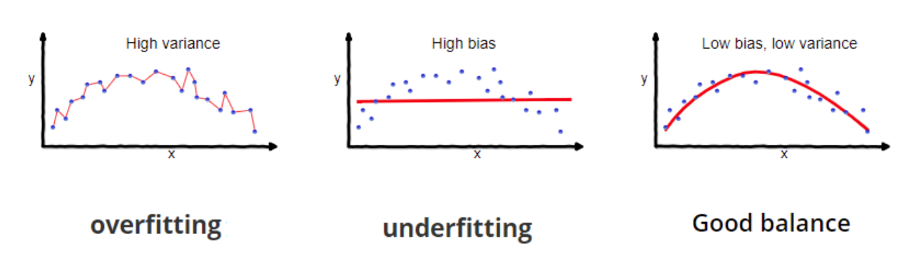
To build a good model, we need to find a good balance between bias and variance such that it minimizes the total error.
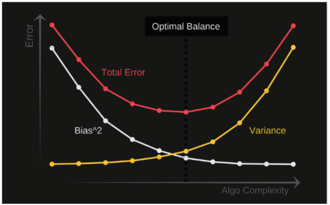
1.2 What is the curse of dimensionality?
If we have more features than observations then we run the risk of massively overfitting our model — this would generally result in terrible out of sample performance.
High-Dimensionality = Sparsity, Sparsity = Error. For example, the K observations that are nearest to a given test observation \(x_{0}\), it may be very far away from \(x_{0}\) in p-dimensional space when p is large, leading to a very poor prediction of f. Machine learning’s basic strategy is to make inferences by looking at similar data.
If the distances are all approximately equal, then all the observations appear equally alike (as well as equally different), and no meaningful information can be formed.
1.3 What is Multi-Collinearity? Why is it an issue?
1.4 How do you detect multicollinearity in Model Data?
1.5 What are the remedies of problem of Multi-collinearity?
1.6 What are Outliers? Leverage & Influential points?
Outliers:
Leverage:
Influence Point:
Cook's Distance: how much the parameter estimates change when a point is removed from the calculations
\[ \frac{1}{n} + \frac{(X_{i}-\bar{X})^2}{SS_{XX}} \]
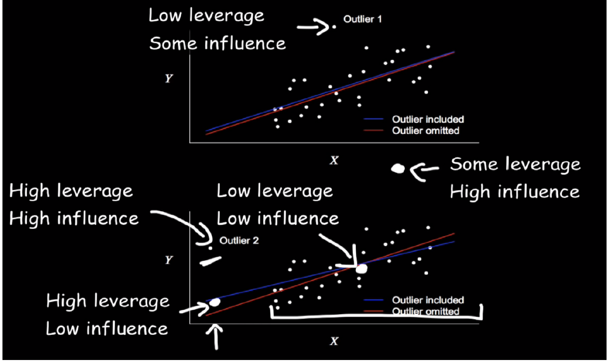
1.7 How can we deal with Outliers?
1.8 Why do you need Cross-Validation?
1.9 How to detect overfitting?
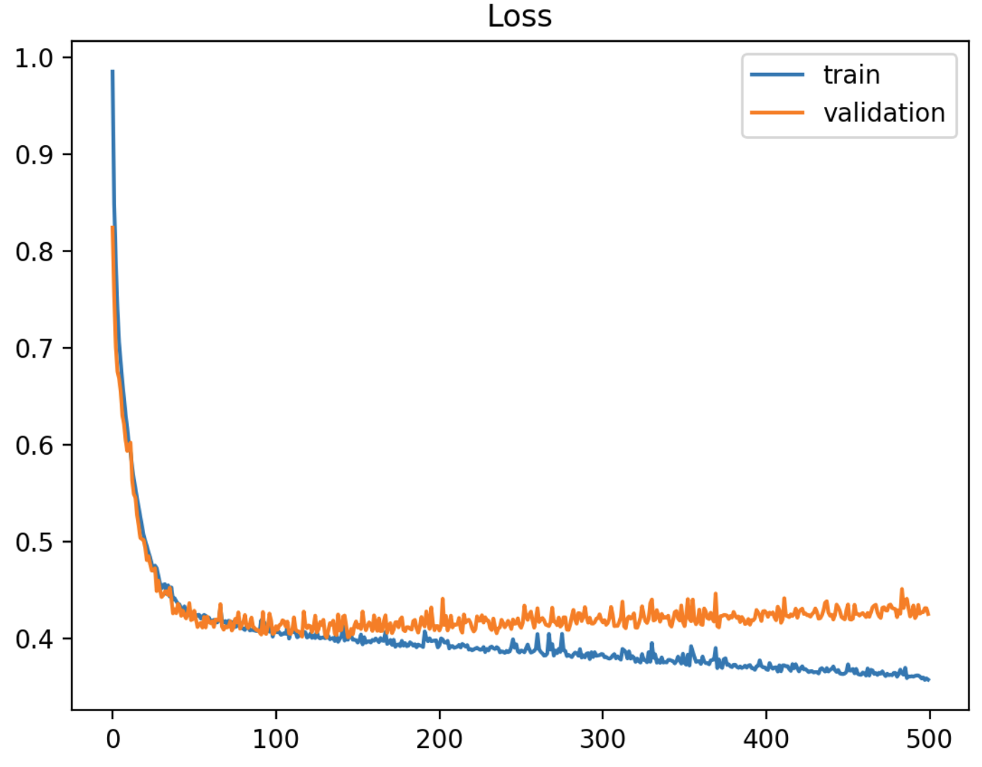
1.10 How do you handle overfitting problem?
1.11 What are the types of missing data? How to handle missing data?
Types of missing data:
Missing data Completely at Random (MCAR):Handle missing data:
Delete: you can drop variables if the data is missing like for more than 60% observations.
Impute: mean, median or mode is a very basic imputation method (rolling window or overall); predict the missing values with other independent variables using random forest. For categorical data, we can treat the missing values as a separate category by itself.
Mean or Medium imputation:
Mode imputation:
Missing category imputation:
Missing indicator:
1.12 You have a train-set, a dev-set and a test-set, how did you manage the distribution of those sets?
1.13 How to handle imbalanced data?
1.14 What are the methods for over-sampling?
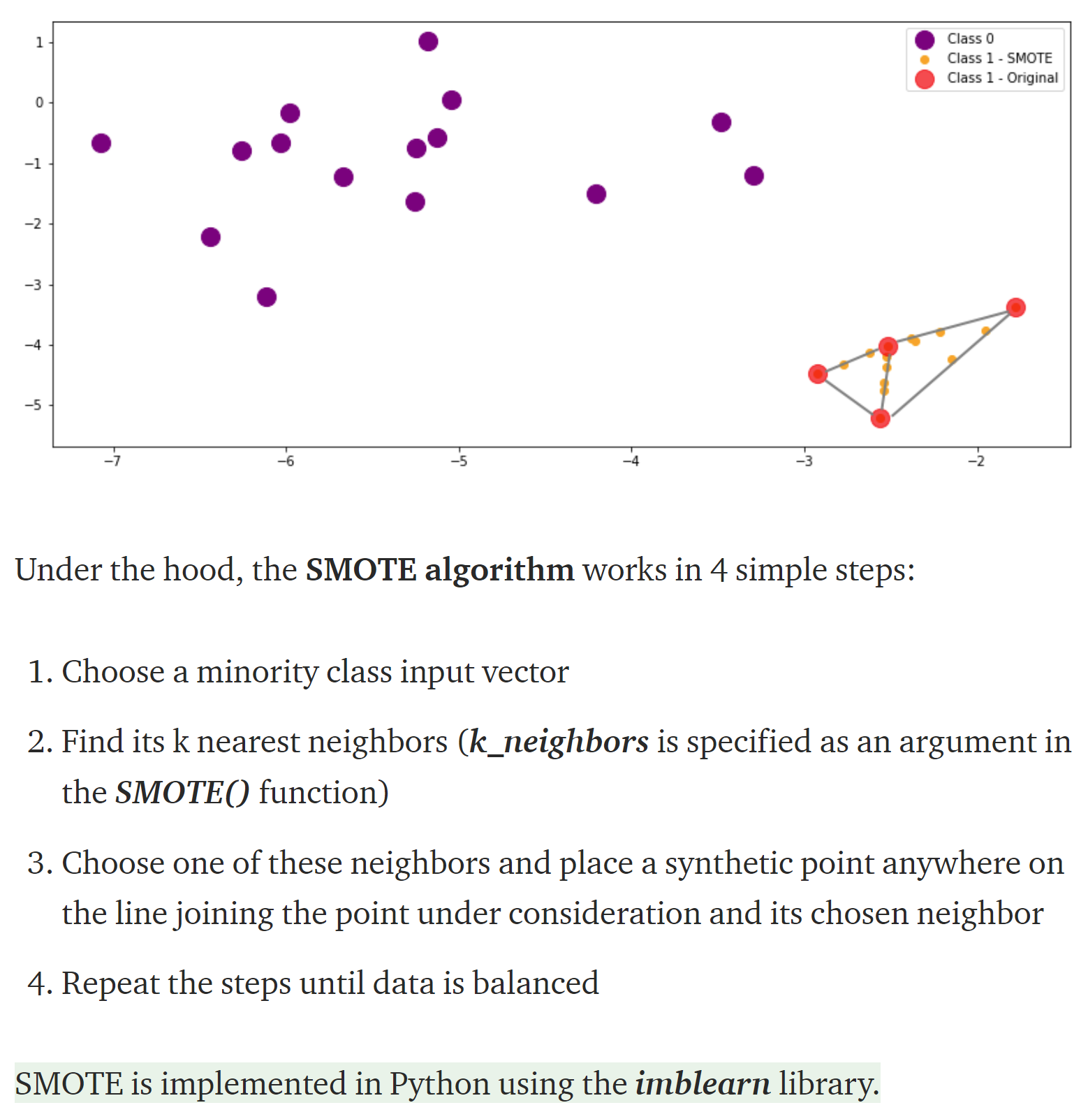
1.15 What is Confusion Matrix? What’s TP, TN, FP, FN, Precision and Recall?
1.16 What is ROC and AUC?
Advantages of using ROC and AUC:
1.17 What are the different types of variables? How to handle categorical variables?
Types of Variables:
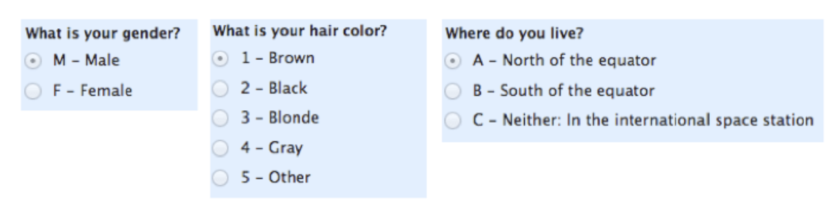
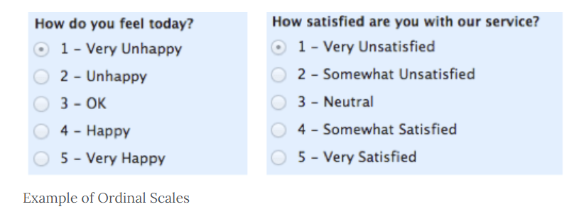
1.18 Are rare labels in a categorical variable a problem?
Rare values can add a lot of information or none at all. For example, consider a stockholder meeting where each person can vote in proportion to their number of shares. One of the shareholders owns 50% of the stock, and the other 999 shareholders own the remaining 50%. The outcome of the vote is largely influenced by the shareholder who holds the majority of the stock. The remaining shareholders may have an impact collectively, but they have almost no impact individually.
The same occurs in real life datasets. The label that is over-represented in the dataset tends to dominate the outcome, and those that are under-represented may have no impact individually, but could have an impact if considered collectively.
More specifically,
**Note** Sometimes rare values, are indeed important. For example, if we are building a model to predict fraudulent loan applications, which are by nature rare, then a rare value in a certain variable, may be indeed very predictive. This rare value could be telling us that the observation is most likely a fraudulent application, and therefore we would choose not to ignore it.
1.19 Why cardinality can cause overfitting?
The number of different labels is known as cardinality
For highly cardinal variables, some labels may appear only in train set then over-fitting, some labels may appear only in test set, then model will not know how to interpret the values
1.20 What is the difference between Generative models and Discriminative models?
A Discriminative model models the decision boundary between the classes.
A Generative Model models the actual distribution of each class.
Section 2. Linear Regression
2.1 What are the basic concepts? What problem does it solve?
Basic Concept: linear regression is used to model relationship between continuous variables. Xs are the predictor, explanatory, or independent variable. Y is the response, outcome, or dependent variable.
2.2 What are the assumptions?
2.3 What if the errors are not normally distributed?
If the erros are not Gaussian distribution, we can still use linear regression, the only thing that is gonna be different is what you use for calculating coefficients, the calculating formula is biased if the errors are not normally distributed, because you are minimizing the MSE, if the errors are not Gaussian, then the maximum likelihood coefficients are not necessary the ones that come to minimize the MSE, you can still use linear regression.
2.4 What are the differences between erros and residuals?
2.5 How to implement Linear Regression?
We want to find the best fit line: \[\hat{y_i} = b_0 + b_1 * x_i \]
We can achieve that by using least squares estimation, which minimizes the sum of the squared predicted errors.
We need to find the values of \( b_0\) and \( b_1\) that minimize:\[Q = \sum_{i=1}^{n} (y_i-\hat{y_i})^2 \] such that \[b_1 = \frac{\sum_{i=1}^{n}(x_i-\bar{x})(y_i-\bar{y})}{\sum_{i=1}^{n}(x_i-\bar{x})^2} \] and \[ b_0 =\bar{y}- b_1\bar{x} \]
B1 = covariance(x, y) / variance(x)
B0 = mean(y) - B1 * mean(x)
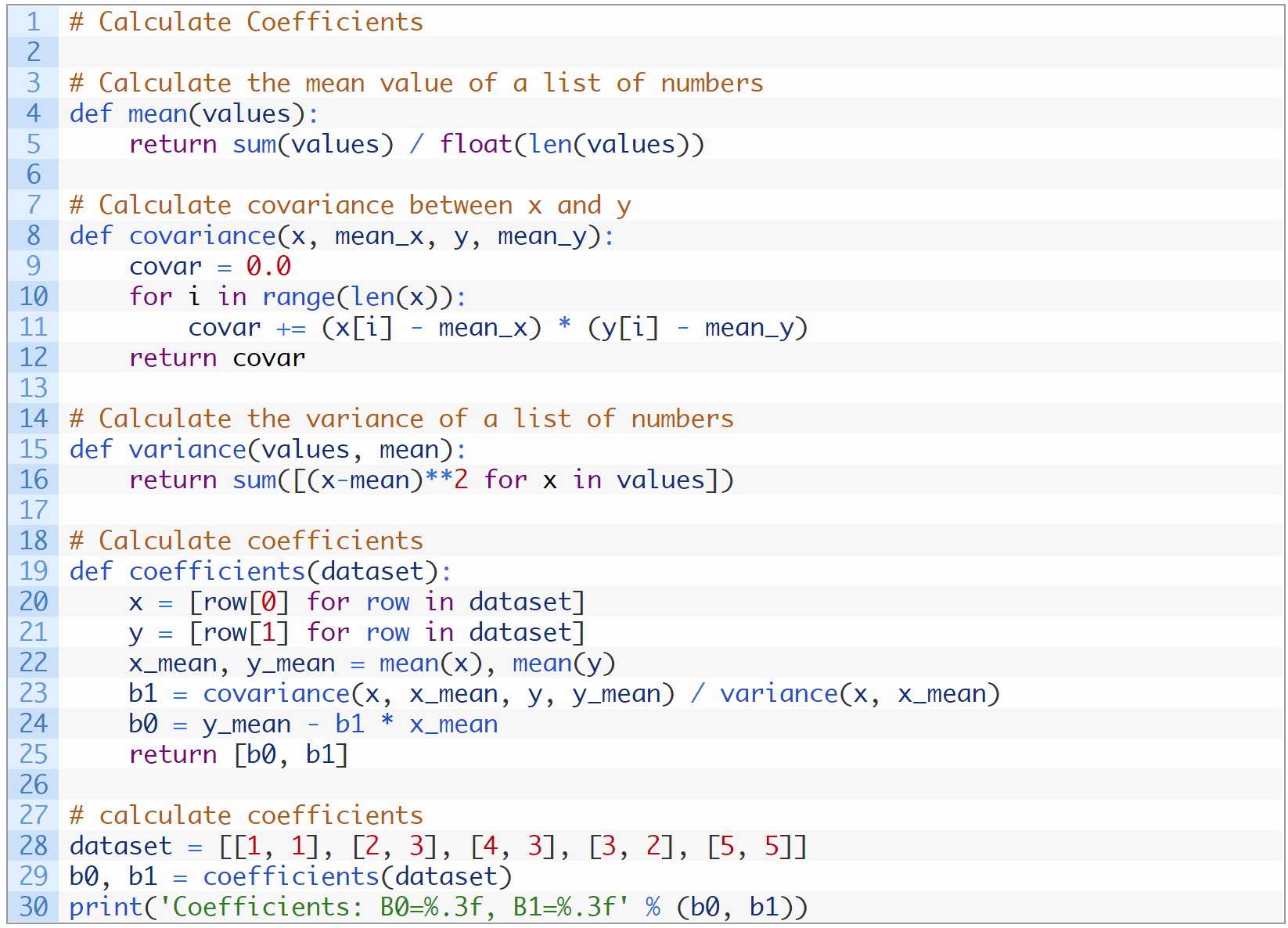
2.6 What is the cost function of Linear regression?
\[ MSE = \frac{1}{n}\sum_{i=1}^{n} (y_i-\hat{y_i})^2 \]
2.7 If you have a set of data and do regression, what if you duplicate all the data and do regression on the new data set?
The mean and variance of the sample would not change therefore the beta estimation would be the same. The standard error will go down. However, since the sample size is doubled this will result in the lower p-value for the beta (from central limit theorem, the standard deviation of the sample mean = standard deviation of population / sqrt(n). This tells us that by simply doubling/duplicating the data, we could trick the regression model to have smaller confidence interval.
2.8 What is R^2?
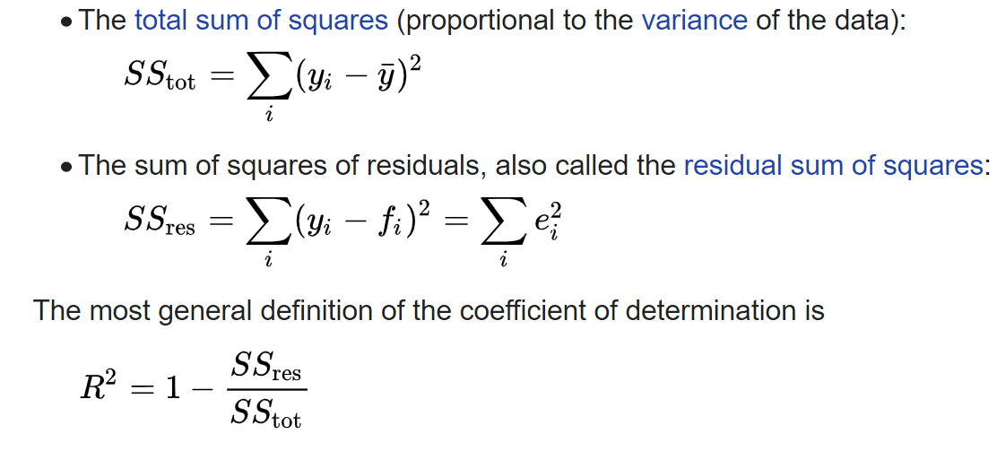
2.9 What Is the Adjusted R-squared?
The adjusted R-squared compares the explanatory power of regression models that contain different numbers of predictors.
Suppose you compare a five-predictor model with a higher R-squared to a one-predictor model. Does the five predictor model have a higher R-squared because it’s better? Or is the R-squared higher because it has more predictors? Simply compare the adjusted R-squared values to find out! The adjusted R-squared is a modified version of R-squared that has been adjusted for the number of predictors in the model. The adjusted R-squared increases only if the new term improves the model more than would be expected by chance. It decreases when a predictor improves the model by less than expected by chance. The adjusted R-squared can be negative, but it’s usually not. It is always lower than the R-squared.
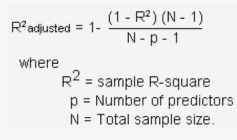
2.10 What’s Gradient Descent?
Gradient Descent is an optimization algorithm that helps machine learning models converge at a minimum value through repeated steps. Essentially, gradient descent is used to minimize a function by finding the value that gives the lowest output of that function. Often times, this function is usually a loss function.
2.11 How to implement Gradient Descent?
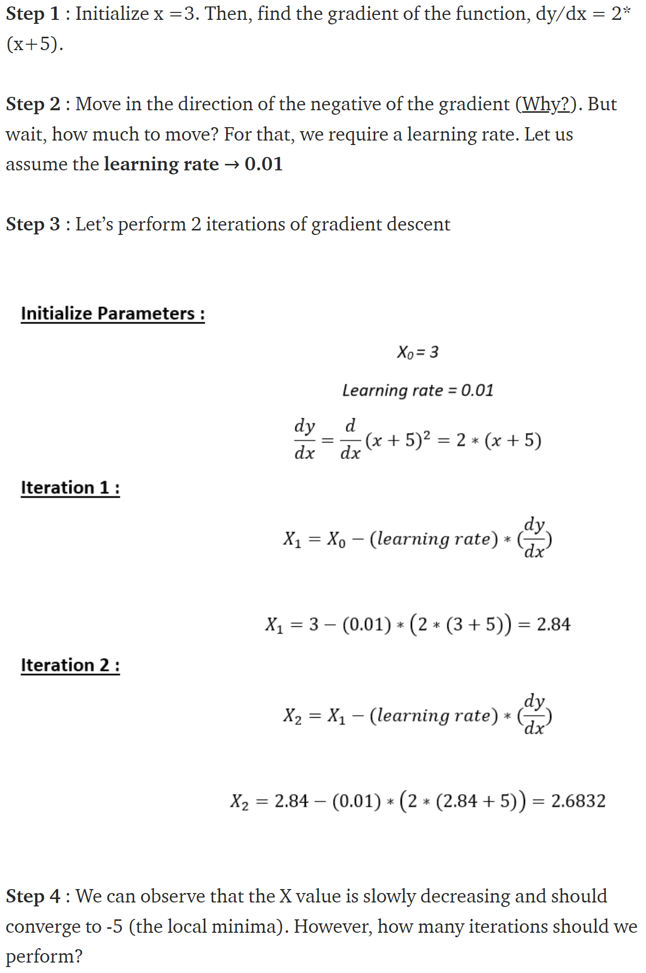
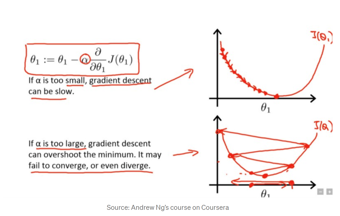
2.12 What’s the difference between confidence interval and predicted interval?
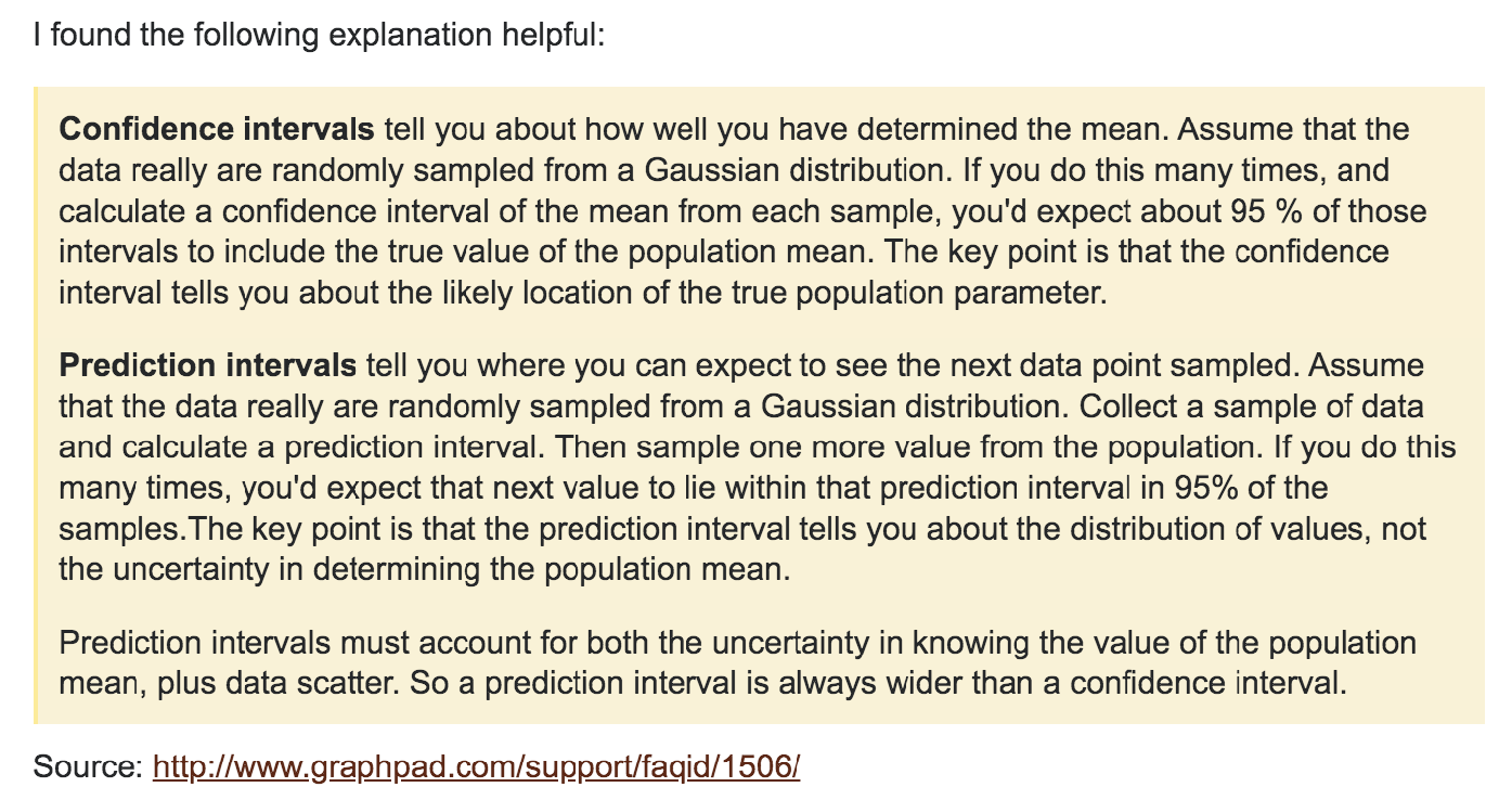
2.13 What are the Advantages/Disadvantages of Linear regression?
Pros:
Cons:
Section 3. Regression with Lasso
3.1 What are the basic concepts of Lasso? What problem does it solve?
Lasso is not a type of model, it is a regularization method for selecting variables and shrinking coefficients to adjust for complexity.
Lasso uses an L1 penalty when fitting the model using least squares
It can force regression coefficients to be exactly 0
When \(\lambda = 0\), then the lasso simply gives the least squares fit
When \(\lambda\) becomes sufficiently large, the lasso gives the null model in which all coefficient estimates equal 0
3.2 What is regularization?
3.3 How to implement Lasso?
Lasso uses L1-the sum of the absolute values of the coefficients
3.4 What is the cost function of Lasso?
$$\hat{\beta}{^{lambda}} = \arg\min_{\beta} \{\sum_{i=1}^{n} (y_i-\beta_0-\sum_{j=1}^{p}x_{ij}\beta_j)^2 + \lambda\sum_{j=1}^{p}||\beta_j|| \}$$
3.5 What are the Advantages/Disadvantages of Lasso?
Pros:
Cons:
3.6 Why does Lasso can coefficients to 0 but Ridge can’t?
The residual sum of squares has elliptical contours, centered at the full least squares estimate. The constraint region for ridge regression is the disk β¹² + β²² ≤ t, while that for lasso is the diamond |β1| + |β2| ≤ t.
Both methods find the first point where the elliptical contours hit the constraint region. Unlike the disk, the diamond has corners; if the solution occurs at a corner, then it has one parameter βj equal to zero. When p > 2, the diamond becomes a rhomboid, and has many corners, flat edges and faces; there are many more opportunities for the estimated parameters to be zero.
Section 4. Regression with Ridge
4.1 What are the basic concepts of Ridge? What problem does it solve?
Ridge uses an L2 penalty when fitting the model using least squares
When lambda = 0, the penalty term has no effect, and ridge regression will produce the least squares estimates.
When lambda become infinite large, the impact of the shrinkage penalty grow, and the ridge regression coefficient estimates will approach to 0.
4.2 How to implement Ridge?
Ridge uses L2-the sum of the squares of the coefficients, can't zero coefficients, force the coefficients to be relatively small.
4.3 What is the cost function of Ridge?
$$\hat{\beta}{^{ridge}} = \arg\min_{\beta} \{\sum_{i=1}^{n} (y_i-\beta_0-\sum_{j=1}^{p}x_{ij}\beta_j)^2 + \lambda\sum_{j=1}^{p}\beta_j^2 \}$$
4.4 What are the Advantages/Disadvantages of Ridge?
Pros:
Cons:
4.5 What is lambda \( \lambda\)?
\( \lambda\)-Lambda is the tuning parameter that decides how much we want to penalize the flexibility of our model
As lambda increases, the impact of the shrinkage penalty grows, and the ridge regression coefficient estimates will approach zero.
Selecting a good value of lambda is critical, cross validation comes in handy for this purpose, the coefficient estimates produced by this method are also known as the L2 norm.
Section 5. Logistic Regression
5.1 What are the basic concepts of Logistic regression? What problem does it solve?
Logistic Regression: is a classification method, usually do binary classification 0 or 1.
A logistic model is one where the log-odds of the probability of an event is a linear combination of independent or predictor variables
5.2 What are the assumptions of Logistic regression?
5.3 How to implement Logistic regression?
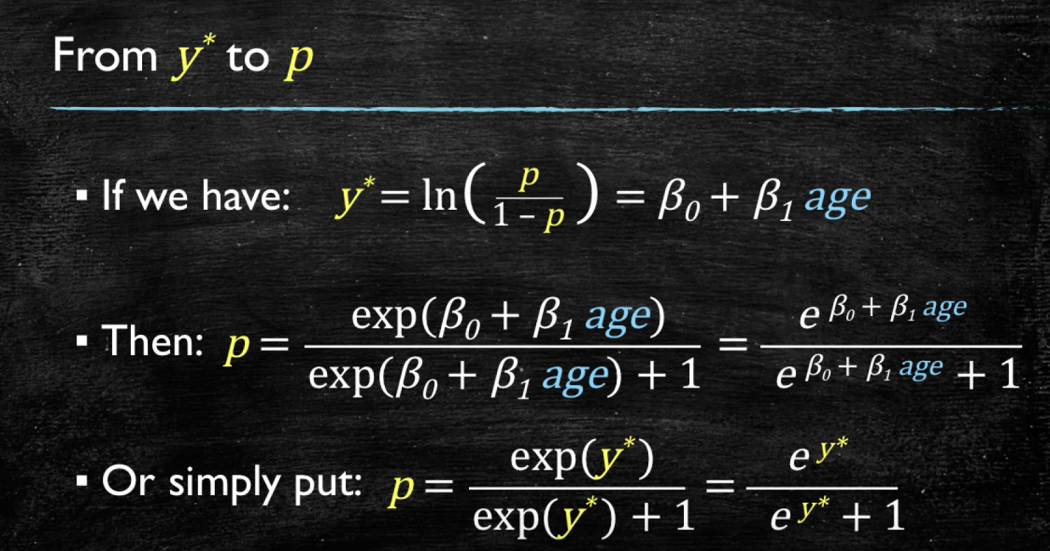
5.4 What is the cost function of Logistic regression?
We use a cost function called Cross-Entropy, also known as Log Loss. Cross-entropy loss can be divided into two separate cost functions: one for y=1 and one for y=0.
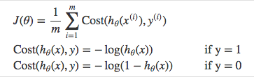
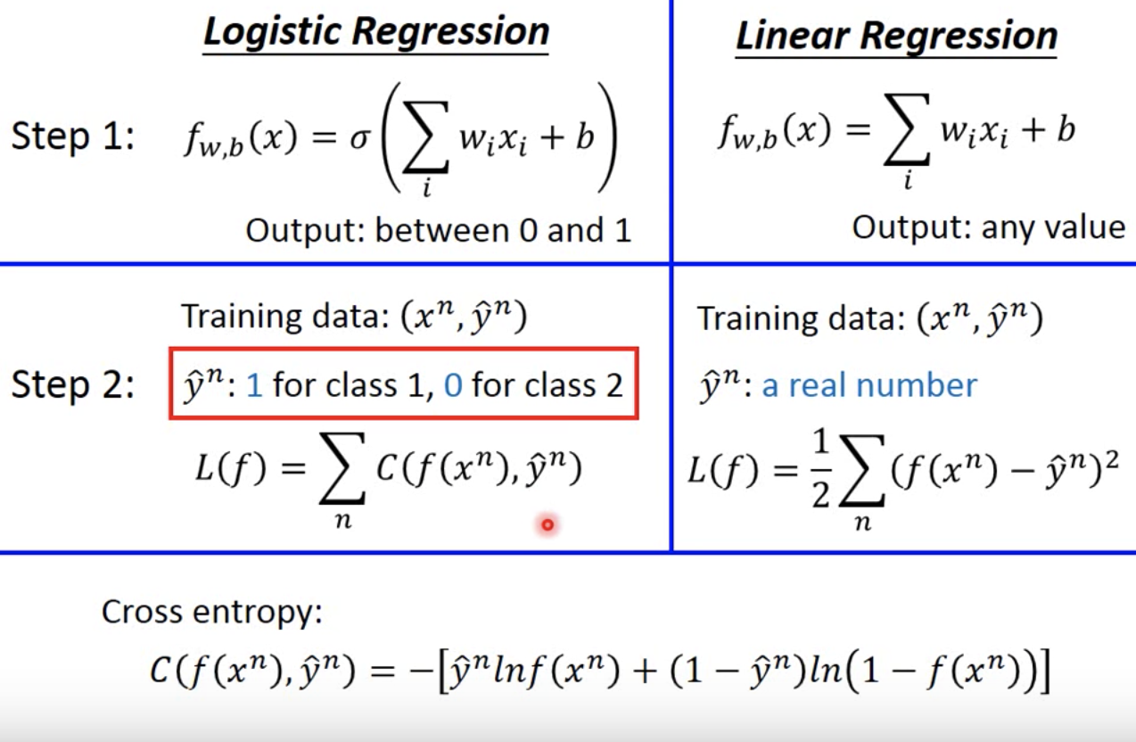
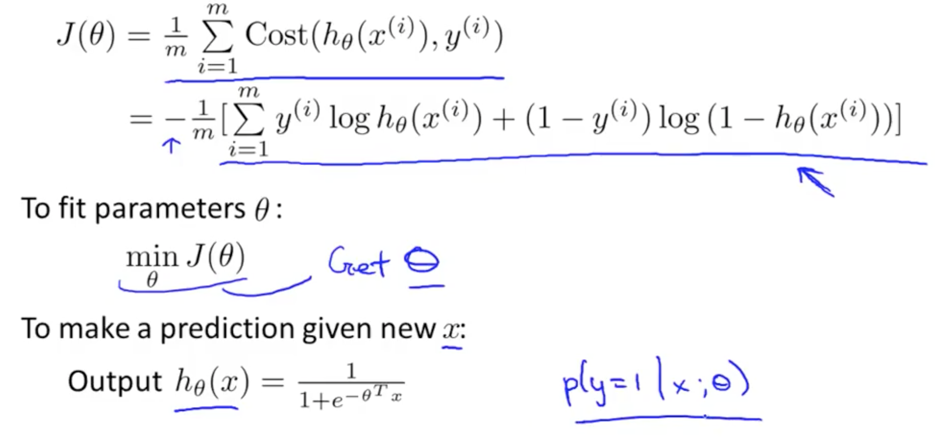
Cost function is achieved by maximum likelihood. We try to find beta0 and beta1 such that plugging these estimates into the model for p(x), yields a number close to one for all individuals who defaulted (class 1), and a number close to 0 for all individuals who did not (class 0).
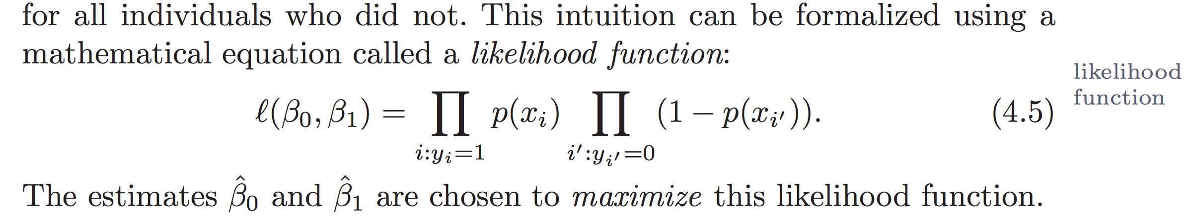
The difference between the cost function and the loss function: the loss function computes the error for a single training example; the cost function is the average of the loss function of the entire training set.
5.5 What are the Advantages/Disadvantages of Logistic regression?
Pros:
Cons:
Section 6. Naïve Bayes
6.1 What are the basic concepts of Naïve Bayes? What problem does it solve?
The Naïve Bayes Algorithm is a Machine Learning algorithm for classification problems. It is primarily used for text classification, which involves high-dimensional training datasets. A few examples are spam filtration, sentimental analysis, and classifying news articles
This algorithm learns the probability of an object with certain features belonging to a particular group in class, in short it is a probabilistic classifier.
6.2 What are the assumptions of Naïve Bayes?
The Naïve Bayes algorithm is called “naïve” because it makes the assumption that the occurrence of a certain feature is independent of the occurrence of other features.
For instance, if you are trying to identify a fruit based on its color shape and taste then an orange colored spherical and tangy fruit would most likely be an orange even if these features depend on each other or on the presence of the other features all these properties individually contribute to the probability that this fruit is an orange and that is why its called Naïve
6.3 What is Bayes' Theorem?
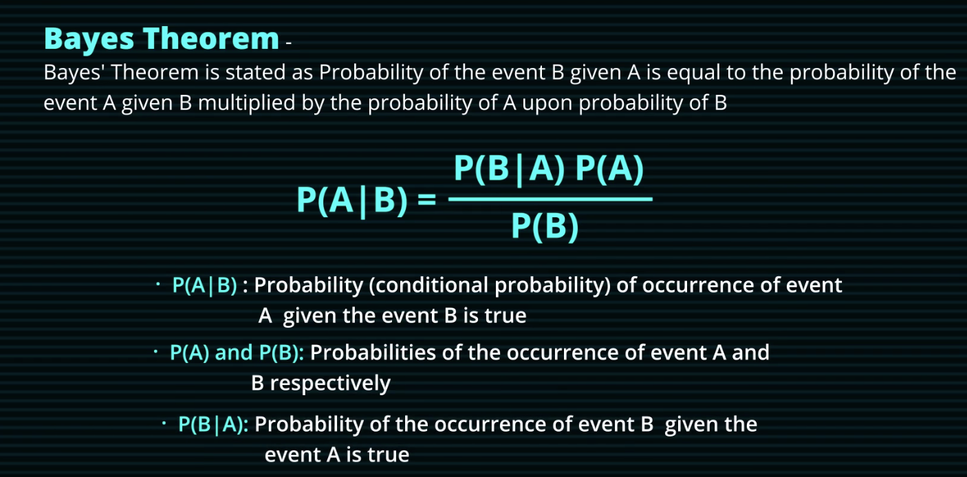
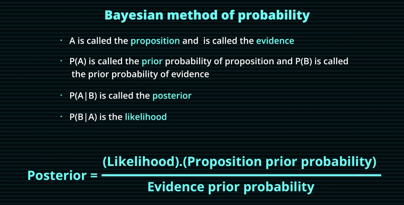
6.4 How to implement Naïve Bayes?
Example 1:
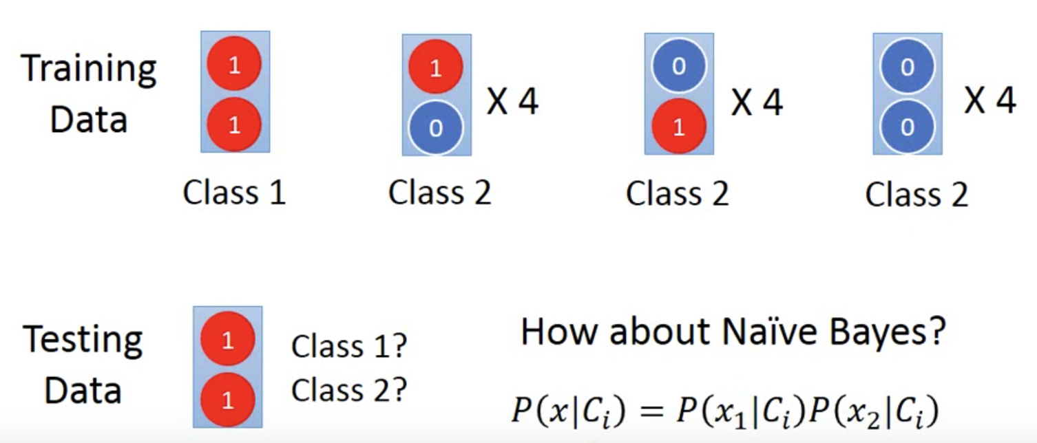
There are total 13 observations in a training dataset:
You are privided one testing data: the two features are both 1.
The Question is: Do you think this testing data belongs to class 1 or class 2?
A lot of people will say it belongs to class 1 by instinct.
Let's see what we can get by using Naive Bayes:
Step 1: Assume independent
Assume the events are independent, so \(P(x) = P(x_1 and x_2) = P(x_1)P(x_2)\), therefore \[P(x|C_i) = P(x_1|C_i)P(x_2|C_i)\]
Step 2: Calculate prior and likelihood
\( P(C_1) = \frac{1}{13}, P(C_2) = \frac{12}{13} \) because there are total 13 observations, only 1 observation labled class 1 and the other 12 labled class 2
\( P(x_1|C_1) = 1, P(x_2|C_1) = 1 \) because both features x1 and x2 are 1 in class 1
So \( P(x|C_1) = P(x_1|C_1)P(x_2|C_1) = 1 \)
\( P(x_1|C_2) = \frac{1}{3} \) because in class 2, there four 1s in the first feature x1, the other eight are 0 (total 12)
\( P(x_2|C_2) = \frac{1}{3} \) because in class 2, there four 1s in the second feature x2, the other eight are 0 (total 12)
So \( P(x|C_2) = P(x_1|C_2)P(x_2|C_2) = \frac{1}{9} \)
Step 3: Bayes Theorem
\( P(C1|x) = \frac{ P(x|C_1)P(C_1) }{P(x)} = \frac{ P(x|C_1)P(C_1) }{P(x|C_1)*P(C_1)+P(x|C_2)*P(C_2)} \)
\( P(C1|x) = \frac{ 1*\frac{1}{13} }{1*\frac{1}{13} +\frac{1}{9}*\frac{12}{13} } = \frac{3}{7} < 0.5 \)
\( P(C2|x) = \frac{ \frac{1}{9} *\frac{12}{13} }{1*\frac{1}{13} +\frac{1}{9}*\frac{12}{13} } = \frac{4}{7} > 0.5 \)
Therefore, based on Naive Bayes, we classify the testing data as class 2
6.5 What is the cost function of Naïve Bayes?
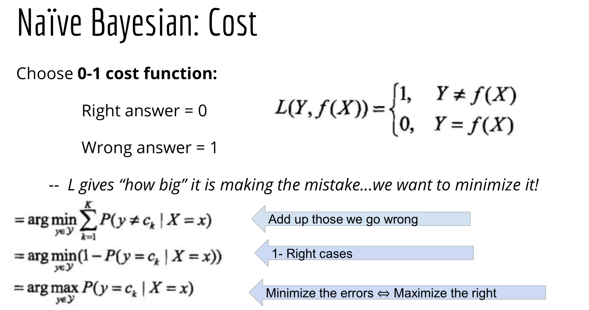
6.6 What are the Advantages/Disadvantages of Naïve Bayes?
Pros:
Cons:
6.7 What are the variations of Naive Bayes?
6.8 What are the applications of Naive Bayes?
Section 7. K-Nearest Neighbors
7.1 What are the basic concepts? What problem does it solve?
K-Nearest Neighbors: Given N training vectors, KNN algorithm identifies the K nearest neighbor of ‘c’, regardless of labels
7.2 What are the steps of the algorithm? What is the cost function?
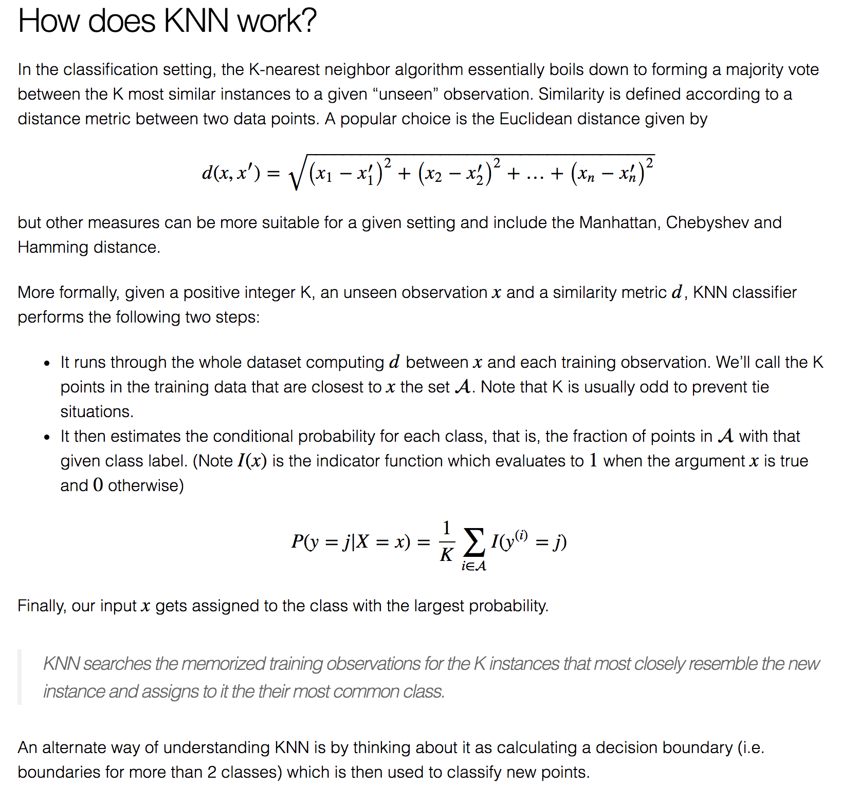
7.3 What are the Advantages/Disadvantages?
Pros:
Cons:
Section 8. K-means Clustering
8.1 What are the basic concepts? What problem does it solve?
K-means is the most popular and widely used clustering method. It is essentially an optimization problem. It is an unsupervised learning. K-means is an iterative algorithm and it does two things, first is a cluster assignment step and second is a move centroid step.
Clustering Assignment step: it goes through each of the example, depending on whether it is closer to some cluster centroid (say k=2), it is going to assign the data points to one of the two cluster centroids.
Move Centroid step: compute the average of all the points that belong to each centroid, and then move the centroid to the average point location.
8.2 What are the assumptions?
Data has to be numeric not categorical.
8.3 What are the steps of the algorithm?
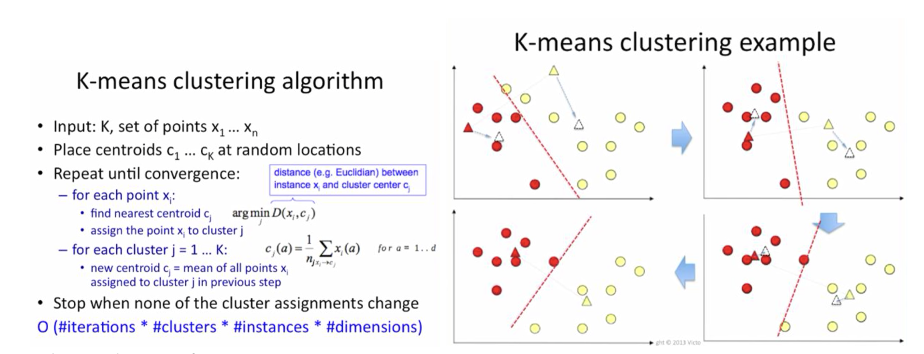
8.4 What is the cost function?
Input: Finite set \(S \subset R{^{d}}\); integer k
Output: \(T \subset R{^{d}}\) with \(|T| = k\)
Goal: Minimize Squared Distance $$Cost(T) = \sum_{x \in S} \min_{z \in T} ||x-z||^2 $$
8.5 What are the Advantages/Disadvantages?
Pros:
Cons:
Section 9. Decision Tree
9.1 What are the basic concepts? What problem does it solve?
9.2 What are the steps of the algorithm?
How to implement a Regression Tree?
How to Implement a Classfication Tree?
9.3 What is the cost function?
Regression Tree: minimize RSS $$\sum_{j=1}^{J} \sum_{i \in R_{j}} (y_{i}-\hat{y}_{R_j})^2 $$
Classification Tree: minimize classification error rate $$E_R = \min_{y} \frac{1}{N_R} \sum_{1:X_i \in R}I(y_i \neq y) $$
9.4 What are the Advantages/Disadvantages?
Pros:
Cons:
Section 10. Random Forest
10.1 What are the basic concepts? What problem does it solve?
Random Forests or random decision forests are an ensemble learning method for classification, regression and other tasks, that operate by constructing a multitude of decision trees at training time and outputing the class that is the mode of the classes (classification) or mean prediction (regression) of the individual trees.
10.2 What are the steps of the algorithm?
Randm Forest is applying bagging to the decision tree:
10.3 What is the cost function?
The same as Decision Tree.
10.4 What are the Advantages/Disadvantages?
Pros:
Cons:
Section 11. Ada-Boost
11.1 What are the basic concepts? What problem does it solve?
It focuses on classification problems and aims to convert a set of weak classifiers into a strong one.
It retrains the algorithm iteratively by choosing the training set based on accuracy of previous training.
The weight-age of each trained classifier at any iteration depends on the accuracy achieved.
Aggregates weak hypotheses for strength; Scale up incorrect, scale down correct; Two heads are better than one, theoretically.
11.2 What are the steps of the algorithm?
11.3 What is the cost function?
Exponential Loss:$$L(y,f(x)) = exp(-yf(x)) $$
11.4 What are the Advantages/Disadvantages?
Pros:
Cons:
Section 12. Gradient Boosting
12.1 What are the basic concepts? What problem does it solve?
The main idea of boosting is to add new models to the ensemble sequentially. At each particular iteration, a new weak, base-learner model is trained with respect to the error of the whole ensemble learnt so far.
Gradient boosting is a machine learning technique for regression and classification problems, which produces a prediction model in the form of an ensemble of weak prediction models, typically decision trees.
It builds the model in a stage-wise fashion like other boosting methods do, and it generalizes them by allowing optimization of an arbitray differentiable loss function.
Whereas random forests build an ensemble of deep independent trees, GBMs build an ensemble of shallow and weak successive trees with each tree learning and improving on the previous. When combined, these many weak successive trees produce a powerful “committee” that are often hard to beat with other algorithms.
12.2 What are the steps of the algorithm?
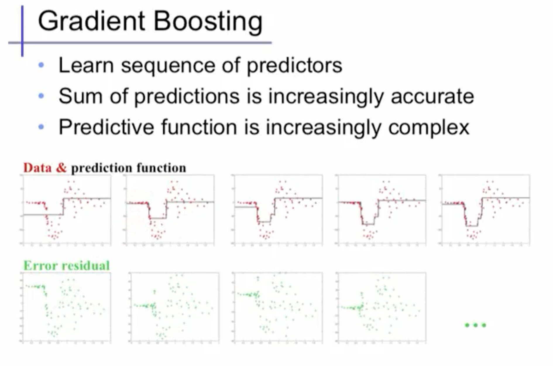
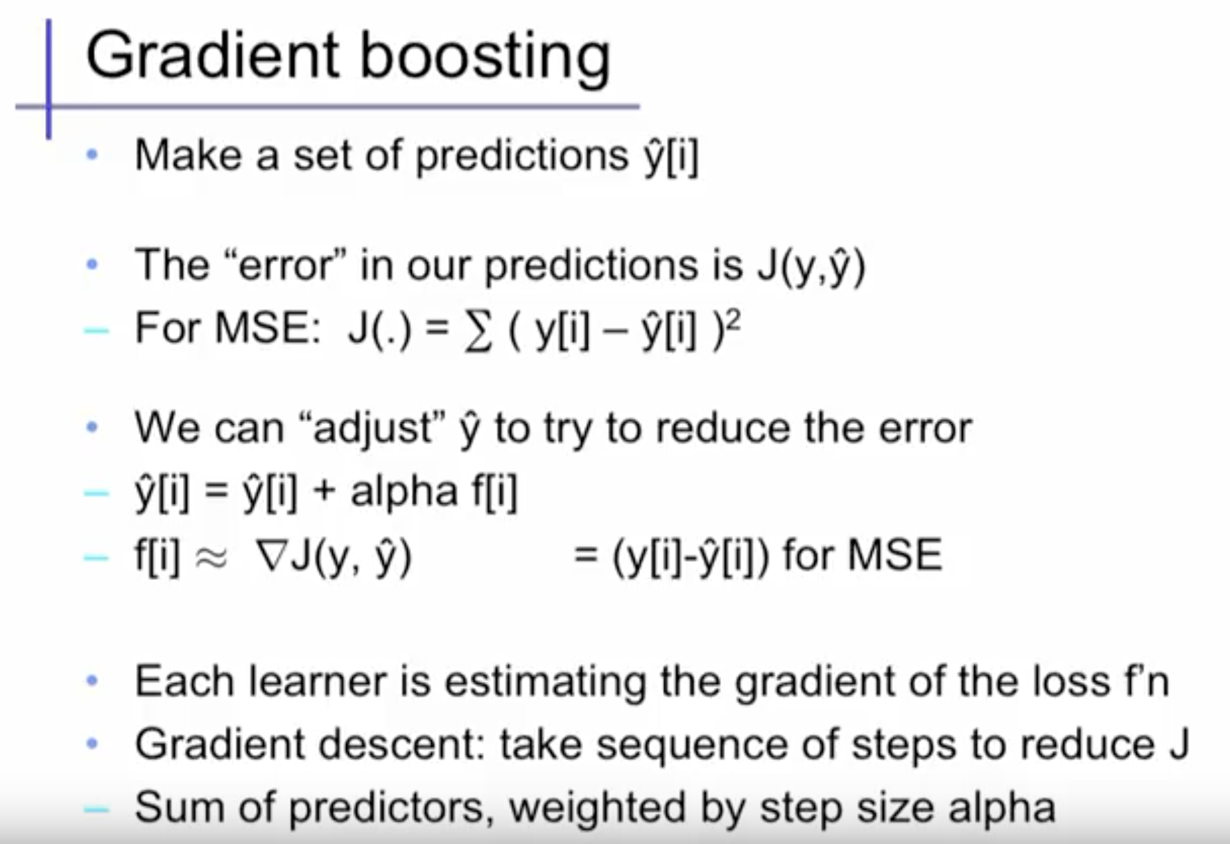
12.3 What is the cost function?
It depends on the model, could be square loss or exponential loss. For any loss function, we can derive a gradient boosting algorithm. Absolute loss and Huber loss are more robust to outliers than square loss.
12.4 What are the Advantages/Disadvantages?
Pros:
Cons:
Section 13. Support Vector Machine (SVM)
13.1 What are the basic concepts? What problem does it solve?
SVM: the goal is to design a hyperplane that classifies all training vectors in 2 classes. The best choice will be the hyperplane that leaves the maximum margin from both classes. As a rule of thumb, SVMs are great for relatively small data sets with fewer outliers.
Hyperplane: is a linear decision surface that splits the space into 2 parts, it is obvious that a hyperplane is a binary classifier. A hyperplane is a p-1 dimension: in two dimensions, a hyperplane is a line, in three dimensions, a hyperplane is a plane.
13.2 What are the steps of the algorithm?
Maximal Margin Hyperplane: is the separating hyperplane for which the margin is largest. If you created a boundary with a large margin with a large buffer zone between the decision boundary and the nearest training data points then you are probably going to do better on the new data.
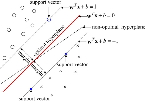
Support Vectors: are the data points nearest to the hyperplane, the points of a dataset that if removed, would alter the position of the dividing hyperplane. Because of this, they can be considered the critical elements of a dataset, they are what help use build our SVM.
Support Vector Classifier: sometimes called a soft margin classifier, rather than seeking the largest possible margin so that every observation is not only on the correct side of the hyperplane but also on the correct side of the margin, we instead allow some observations to be on the incorrect side of the margin, or even incorrect side of the hyperplane.
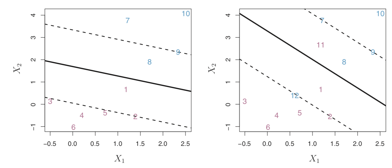
Kernel Trick: the idea is that our data which isn't linearly separable in our n' dimensional space may be linearly separable in a higher dimensional space.
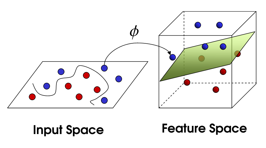
13.3 What is the cost function?
Hinge Loss:
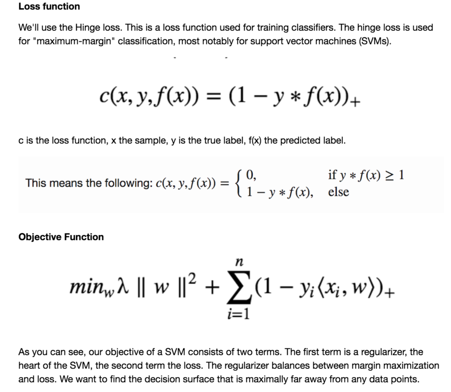
13.4 What are the Advantages/Disadvantages?
Pros:
Cons:
Section 14. Principal Component Analysis (PCA)
14.1 What are the basic concepts? What problem does it solve?
PCA: is a dimension reduction method for compressing a lot of data into something that captures the essence of the original data. It takes a dataset with a lot of dimensions and flattens it to 2 or 3 dimensions so we can look at it. PC1 (the first principal component) is the axis that spans the most variation. PC2 is the axis that spans the second most varation.
PCA: is a tool to reduce multidimensional data to lower dimensions while retaining most of the information. It covers standard deviation, covariance, and eigenvectors.
PCA: is a statistical method that uses an orthogonal transformation to convert a set of observations of correlated variables into a set of values of linearly uncorrelated variables called principal components.
PCA: is a variance maximizing exercise, it projects the original data onto a direction which maximizes variance.
PCAs: are eigen-pairs, they describe the direction in the original feature space with the greatest variances.
PCA: is an orthogonal, linear transformation that transforms data to a new coordinate system such that the greatest variance by some projection of data lies on the first principal component. The second greatest variance lies on the second component. The variance is the measurement of how spread out some data is.
PCA: is a classical featur extraction and data representation technique widely used in the areas of pattern recognization and computer vision such as face recognization.
14.2 What are the assumptions?
14.3 What are the steps of the algorithm?
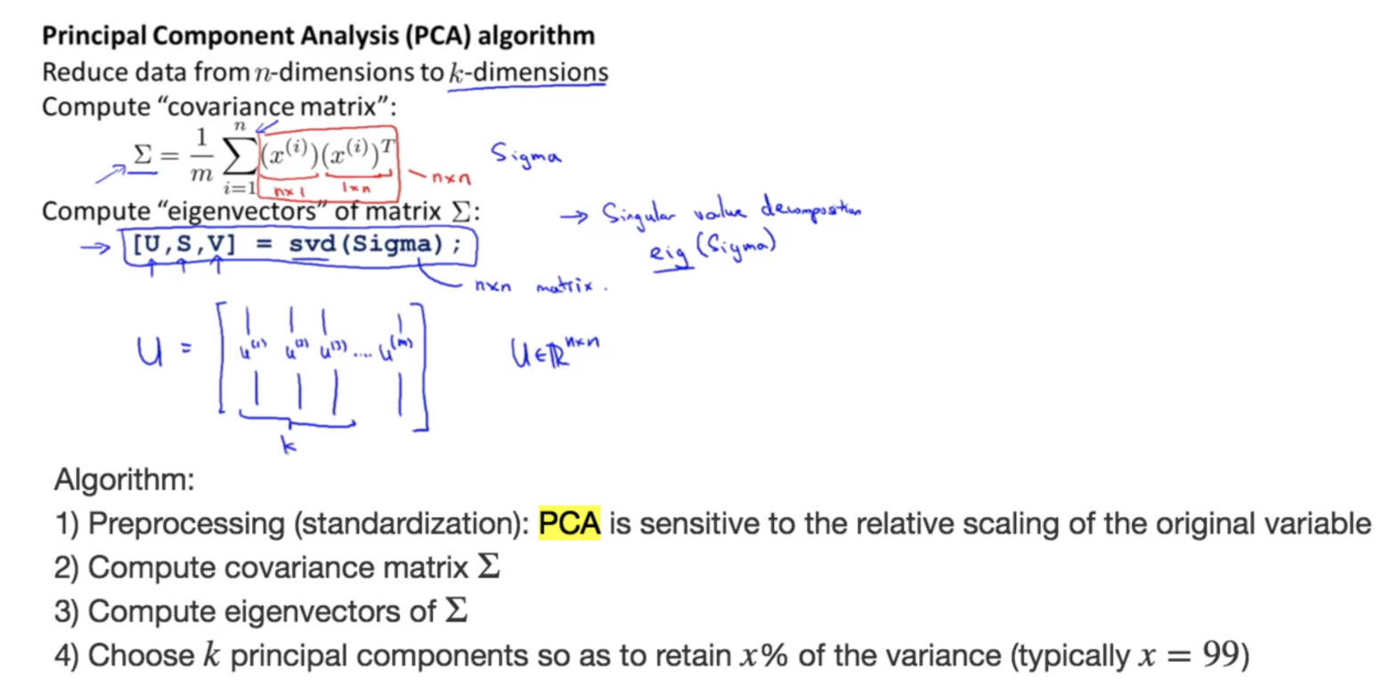
14.4 What is the cost function?
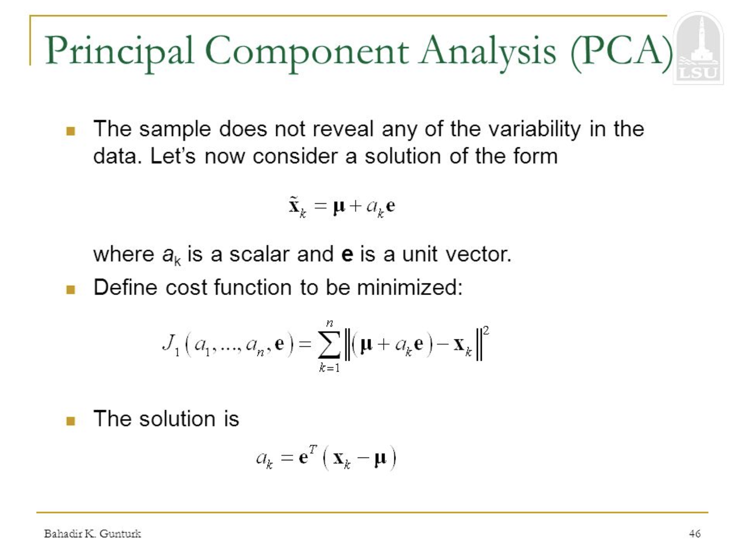
14.5 What are the Advantages/Disadvantages?
Pros:
Cons:
Section 15. Neural Network
15.1 What are the basic concepts? What problem does it solve?
Neural Networks: are computing systems vaguely inspired by the biological neural networks that constitute animal brains. The neural network itself is not an algorithm, but rather a framework for many different machine learning algorithms to work together and process complex data inputs. such systems "learn" to perform tasks by considering examples, generally without being programmed with any task-specific rules. For example, in image recognition, they might learn to identify images that contain cats by analyzing example images that have been manually labled as "cat" or "no cat" and using the results to identify cats in other images. (Wikipedia Definition)
Neuron: a thing that holds a number, specifically a number between 0 and 1
Input Layer: \(x\)
Output Layer: \(\hat{y}\)
Hidden Layer: arbitray
Activation Function: are what connected between hidden layers, it squishes the real number line into the range between 0 and 1, a comon function that does this is called the sigmoid function also known as a logistic curve basically very negative inputs end up close to zero very positive inputs end up close to 1. Activation of the neuron here is basically a measure of how positive the relevant weighted sum is.
Weights and Biases: between each layer \(W\) and \(b\), weights tell you what kind of pattern this neuron in the second layer is picking up on; bias is for inactivity: may be you only want it to be active when the sum is bigger than say 10, that is you want some bias for it to be inactive, just need to add in some number like negative 10 to the weighted sum, before plug it into the sigmoid function, it tells you how high the weighted sum needs to be before the neuron starts getting meaninfully active.
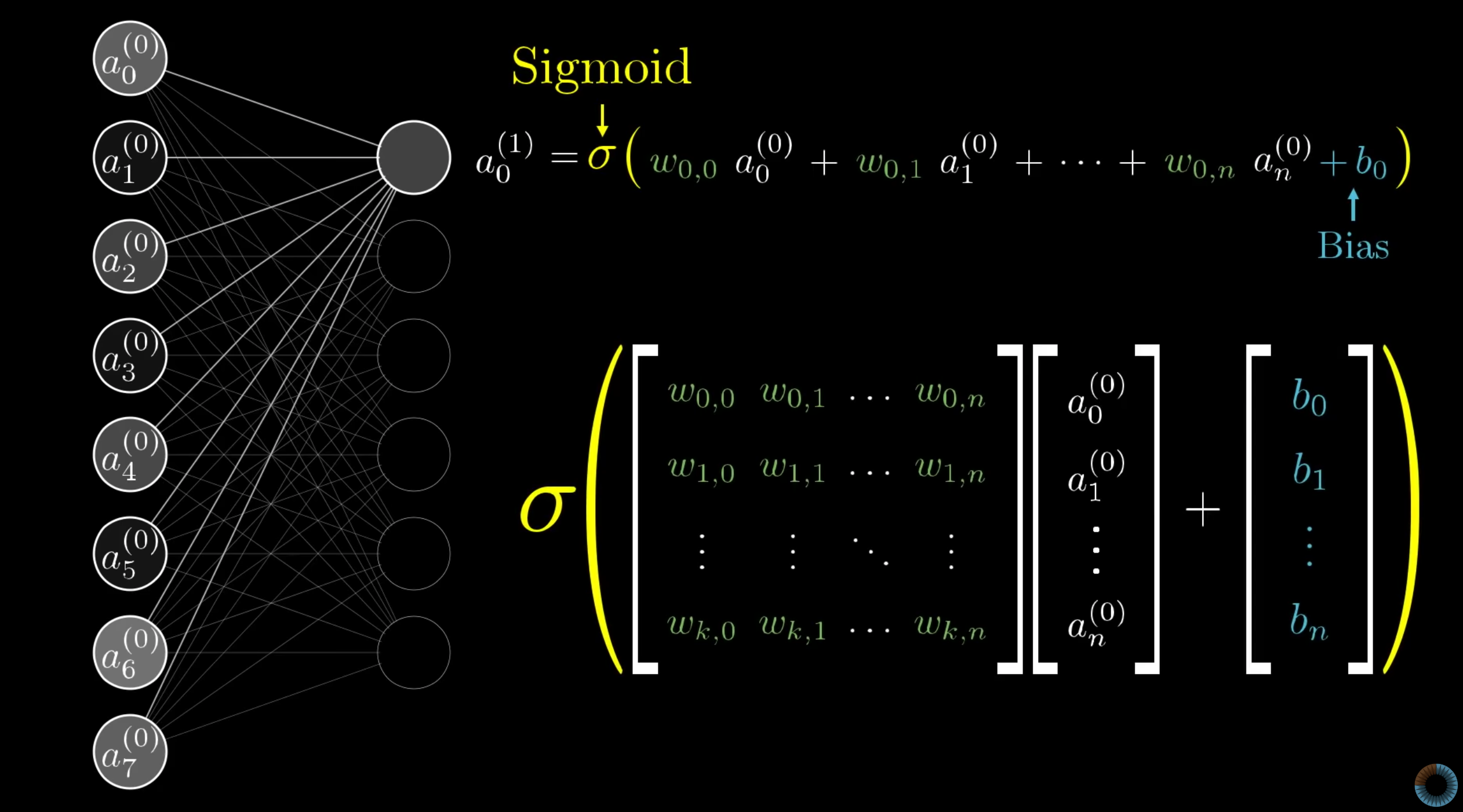
15.2 What are the steps of the algorithm?
Train the Neural Network: the process of fine-tunning the weights and biases from the input data, our goal in training is to find the best set of weights and biases that minimizes the loss function.
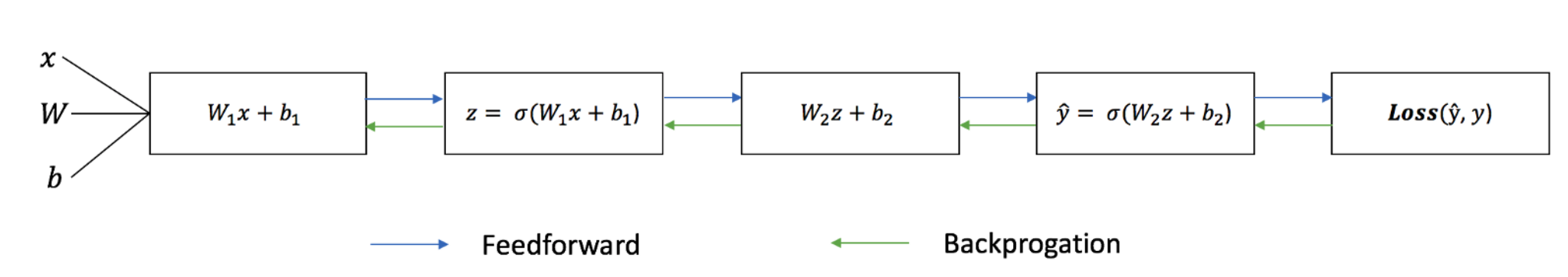
15.3 What is the cost function?
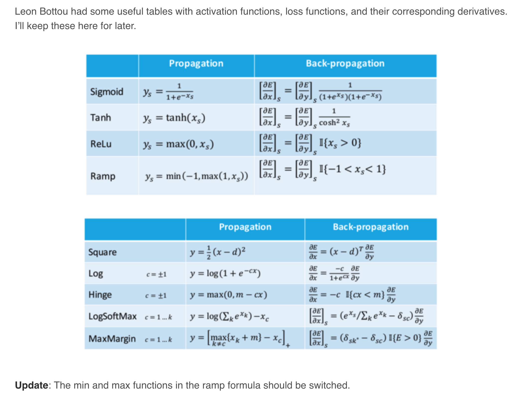
15.4 What are the Advantages/Disadvantages?
Pros:
Cons:
Reference:
Textbook
An Introduction to Statistical LearningLinear Regression
http://r-statistics.co/Assumptions-of-Linear-Regression.htmlLogistic Regression
Video 8: Logistic Regression - Interpretation of Coefficients and Forecasting
Logistic Regression from holehouse
Logistic Regression from ritchieng
Machine Learning Cheatsheet: Logistic Regression
Machine Learning (Hung-yi Lee, NTU) Logistic Regression
How is the cost function from Logistic Regression derivated
ML Lecture 5: Logistic RegressionNaive Bayes
Introduction to Naive Bayes Theorem
6 Easy Steps to Learn Naive Bayes Algorithm
Machine Learning Algorithms Review (Part 2)KNN
A Complete Guide to K-Nearest-Neighbors with Applications in Python and RKmeans
Kmeans Steps from Victor Lavrenko's Youtube VideoRandom Forest
Random Forest Wikipedia
Tree Based Model SummaryAdaboost
Adaptive Boosting by Hsuan-Tien Lin
Ensemble Method by Hung-yi Lee
Boosting algorithm: AdaBoost
Chapter 6: Adaboost ClassifierGBM
Gradient Boosting from scratch
Gradient Boosting Wikipedia
gbm_regression
Ensembles (3): Gradient Boosting by Alexander IhlerSVM
SVM (medium.com)
Kernel trick explanationPCA
Dimensionality Reduction by Andrew Ng
Pattern ClassificationNeural Network
Artificial neural network by Wikipedia
How to build your own Neural Network from scratch in Python
Introduction to Neural Networks, Advantages and Applications
What are the advantages/disadvantages of Artificial Neural networks?
Neural Networks Demystified [Part 1: Data and Architecture] by Welch Labs
Loss Functions in Neural Networks
26 Things I Learned in the Deep Learning Summer School